ABSTRACT Deoxygenation is commonly observed in oceans and lakes but less expected in shallower, flowing rivers. Here we reconstructed daily water temperature and dissolved oxygen in 580

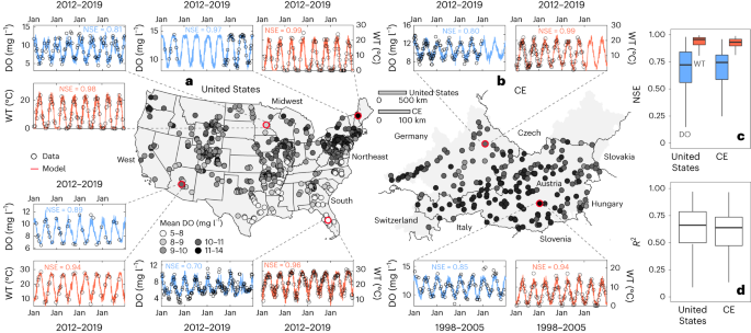
rivers across the United States and 216 rivers in Central Europe by training a deep learning model using temporal weather and water quality data and static watershed attributes (for example,

hydro-climate, topography, land use, soil). Results revealed persistent warming in 87% and deoxygenation in 70% of the rivers. Urban rivers demonstrated the most rapid warming, whereas

agricultural rivers experienced the slowest warming but fastest deoxygenation. Mean deoxygenation rates (−0.038 ± 0.026 mg l−1 decade−1) were higher than those in oceans but lower than those

is a preview of subscription content, access via your institution ACCESS OPTIONS Access through your institution Access Nature and 54 other Nature Portfolio journals Get Nature+, our

best-value online-access subscription $32.99 / 30 days cancel any time Learn more Subscribe to this journal Receive 12 print issues and online access $209.00 per year only $17.42 per issue

Learn more Buy this article * Purchase on SpringerLink * Instant access to full article PDF Buy now Prices may be subject to local taxes which are calculated during checkout ADDITIONAL

ACCESS OPTIONS: * Log in * Learn about institutional subscriptions * Read our FAQs * Contact customer support SIMILAR CONTENT BEING VIEWED BY OTHERS TEMPERATURE OUTWEIGHS LIGHT AND FLOW AS

THE PREDOMINANT DRIVER OF DISSOLVED OXYGEN IN US RIVERS Article 09 March 2023 IMPACT OF CLIMATE CHANGE ON RIVER WATER TEMPERATURE AND DISSOLVED OXYGEN: INDIAN RIVERINE THERMAL REGIMES

Article Open access 02 June 2022 DEEPBASE: A DEEP LEARNING-BASED DAILY BASEFLOW DATASET ACROSS THE UNITED STATES Article Open access 07 January 2025 DATA AVAILABILITY Discharge and water

quality data in the United States were downloaded from the USGS National Water Information System (NWIS) at https://waterdata.usgs.gov/nwis. The historical meteorological datasets in the

United States are available from the NLDAS-2 (https://ldas.gsfc.nasa.gov/nldas/v2/forcing) and DAYMET (https://daymet.ornl.gov). Basin characteristics in the United States are from GAGES-II

archived at https://water.usgs.gov/GIS/metadata/usgswrd/XML/gagesII_Sept2011.xml. The LamaH-CE paper and dataset including meteorological forcing, discharge and basin attributes is available

at https://doi.org/10.5194/essd-13-4529-2021. Due to limits in sharing raw water quality data from providers in the CE region, we recommend accessing data directly from their websites:

Water quality data for Austria were obtained from the Federal Ministry of Agriculture, Regions and Tourism at https://wasser.umweltbundesamt.at/h2odb/fivestep/abfrageQdPublic.xhtml. Water

quality data in Switzerland were obtained from the Swiss Federal Institute of Aquatic Science and Technology (EAWAG) and Federal Office for the Environment (FOEN) at

https://doi.org/10.25678/0004AV. Water quality data for Germany were obtained from the State Agency for the Environment Baden-Württemberg at

https://udo.lubw.baden-wuerttemberg.de/public/index.xhtml, and the Bavarian State Office for the Environment at https://www.gkd.bayern.de/en/rivers/chemistry. Supporting data are deposited

at https://github.com/LiReactiveWater/WT-DO-US-CE-dataset. The projected downscaled forcing data from the NEX-GDDP-CMIP6 database19 can be found at https://doi.org/10.7917/OFSG3345. CODE

AVAILABILITY The deep learning code and instruction are available on GitHub at https://github.com/LiReactiveWater/WT-DO-US-CE-LSTM. The ‘streamMetabolizer’ R package for calculating DO

saturation concentration is available on GitHub at https://github.com/USGS-R/streamMetabolizer. The ‘dataRetrieval’ R package for downloading discharge and water quality data for the United

States is available on GitHub https://github.com/USGS-R/dataRetrieval. The ‘bestNormalize’ R package for transforming model inputs is available on GitHub at

https://github.com/cran/bestNormalize. REFERENCES * Ficklin, D. L. et al. Rethinking river water temperature in a changing, human-dominated world. _Nat. Water_ 1, 125–128 (2023). Article 

Google Scholar  * Rosamond, M. S., Thuss, S. J. & Schiff, S. L. Dependence of riverine nitrous oxide emissions on dissolved oxygen levels. _Nat. Geosci._ 5, 715–718 (2012). Article  CAS

  Google Scholar  * Sundby, B. et al. The effect of oxygen on release and uptake of cobalt, manganese, iron and phosphate at the sediment–water interface. _Geochim. Cosmochim. Acta_ 50,

1281–1288 (1986). Article  CAS  Google Scholar  * Jane, S. F. et al. Widespread deoxygenation of temperate lakes. _Nature_ 594, 66–70 (2021). Article  CAS  Google Scholar  * Breitburg, D. et

al. Declining oxygen in the global ocean and coastal waters. _Science_ 359, eaam7240 (2018). Article  Google Scholar  * Blaszczak, J. R. et al. Extent, patterns, and drivers of hypoxia in

the world’s streams and rivers. _Limnol. Oceanogr. Lett._ https://doi.org/10.1002/lol2.10297 (2022). Article  Google Scholar  * Bernhardt, E. S. et al. The metabolic regimes of flowing

waters. _Limnol. Oceanogr._ 63, S99–S118 (2018). Article  Google Scholar  * Bernhardt, E. S. et al. Light and flow regimes regulate the metabolism of rivers. _Proc. Natl Acad. Sci. USA_ 119,

e2121976119 (2022). Article  CAS  Google Scholar  * Helton, A. M., Poole, G. C., Payn, R. A., Izurieta, C. & Stanford, J. A. Scaling flow path processes to fluvial landscapes: an

integrated field and model assessment of temperature and dissolved oxygen dynamics in a river–floodplain–aquifer system. _J. Geophys. Res. Biogeosci._ https://doi.org/10.1029/2012JG002025

(2012). * Piatka, D. R. et al. Transfer and transformations of oxygen in rivers as catchment reflectors of continental landscapes: a review. _Earth Sci. Rev._ 220, 103729 (2021). Article 

CAS  Google Scholar  * Utz, R. M., Bookout, B. J. & Kaushal, S. S. Influence of temperature, precipitation, and cloud cover on diel dissolved oxygen ranges among headwater streams with

variable watershed size and land use attributes. _Aquat. Sci._ 82, 82 (2020). Article  CAS  Google Scholar  * Hancke, K. & Glud, R. N. Temperature effects on respiration and

photosynthesis in three diatom-dominated benthic communities. _Aquat. Microb. Ecol._ 37, 265–281 (2004). Article  Google Scholar  * Girard, J. _Principles of Environmental Chemistry_ (Jones

& Bartlett Publishers, 2013). * Blaszczak, J. R., Delesantro, J. M., Urban, D. L., Doyle, M. W. & Bernhardt, E. S. Scoured or suffocated: urban stream ecosystems oscillate between

hydrologic and dissolved oxygen extremes. _Limnol. Oceanogr._ 64, 877–894 (2019). Article  CAS  Google Scholar  * Carter, A. M., Blaszczak, J. R., Heffernan, J. B. & Bernhardt, E. S.

Hypoxia dynamics and spatial distribution in a low gradient river. _Limnol. Oceanogr._ 66, 2251–2265 (2021). Article  Google Scholar  * IPCC _Climate Change 2021: The Physical Science Basis_

(eds Masson-Delmotte, V. et al.) (Cambridge Univ. Press, 2021). * Guo, D. et al. A data-based predictive model for spatiotemporal variability in stream water quality. _Hydrol. Earth Syst.

Sci._ 24, 827–847 (2020). Article  Google Scholar  * Zhi, W., Ouyang, W., Shen, C. & Li, L. Temperature outweighs light and flow as the predominant driver of dissolved oxygen in US

rivers. _Nat. Water_ 1, 249–260 (2023). Article  Google Scholar  * Thrasher, B. et al. NASA global daily downscaled projections, CMIP6. _Sci. Data_ https://doi.org/10.1038/s41597-022-01393-4

(2022) * Luterbacher, J. et al. European summer temperatures since Roman times. _Environ. Res. Lett._ 11, 024001 (2016). Article  Google Scholar  * _Climate at a Glance: National Mapping_

(NOAA National Centers for Environmental Information, accessed 13 August 2022); https://www.ncei.noaa.gov/cag/ * van der Schrier, G., van den Besselaar, E. J. M., Klein Tank, A. M. G. &

Verver, G. Monitoring European average temperature based on the E-OBS gridded data set. _J. Geophys. Res. Atmos._ 118, 5120–5135 (2013). Article  Google Scholar  * Thompson, A. M., Kim, K.

& Vandermuss, A. J. Thermal characteristics of stormwater runoff from asphalt and sod surfaces 1. _J. Am. Water Resour. Assoc._ 44, 1325–1336 (2008). Article  Google Scholar  * Kinouchi,

T., Yagi, H. & Miyamoto, M. Increase in stream temperature related to anthropogenic heat input from urban wastewater. _J. Hydrol._ 335, 78–88 (2007). Article  Google Scholar  * Adeola

Fashae, O., Abiola Ayorinde, H., Oludapo Olusola, A. & Oluseyi Obateru, R. Landuse and surface water quality in an emerging urban city. _Appl. Water Sci._ 9, 25 (2019). Article  Google

Scholar  * Daniel, M. H. B. et al. Effects of urban sewage on dissolved oxygen, dissolved inorganic and organic carbon, and electrical conductivity of small streams along a gradient of

urbanization in the Piracicaba River Basin. _Water Air Soil Pollut._ 136, 189–206 (2002). Article  CAS  Google Scholar  * Welker, T. L., Overturf, K. & Abernathy, J. Effect of aeration

and oxygenation on growth and survival of rainbow trout in a commercial serial-pass, flow-through raceway system. _Aquac. Rep._ 14, 100194 (2019). Article  Google Scholar  * Vaquer-Sunyer,

R. & Duarte, C. M. Thresholds of hypoxia for marine biodiversity. _Proc. Natl Acad. Sci. USA_ 105, 15452–15457 (2008). Article  CAS  Google Scholar  * Ice, G. & Sugden, B. Summer

dissolved oxygen concentrations in forested streams of northern Louisiana. _South. J. Appl. Forestry_ 27, 92–99 (2003). Article  Google Scholar  * Whitworth, K. L., Baldwin, D. S. &

Kerr, J. L. Drought, floods and water quality: drivers of a severe hypoxic blackwater event in a major river system (the southern Murray–Darling Basin, Australia). _J. Hydrol._ 450-451,

190–198 (2012). Article  CAS  Google Scholar  * Calleja, M. L., Al-Otaibi, N. & Morán, X. A. G. Dissolved organic carbon contribution to oxygen respiration in the central Red Sea. _Sci.

Rep._ 9, 4690 (2019). Article  Google Scholar  * Zhi, W. et al. From hydrometeorology to river water quality: can a deep learning model predict dissolved oxygen at the continental scale?

_Environ. Sci. Technol._ 55, 2357–2368 (2021). Article  CAS  Google Scholar  * Li, J. & Wong, D. W. S. Effects of DEM sources on hydrologic applications. _Comput. Environ. Urban Syst._

34, 251–261 (2010). Article  Google Scholar  * Preece, R. M. & Jones, H. A. The effect of Keepit Dam on the temperature regime of the Namoi River, Australia. _River Res. Appl._ 18,

397–414 (2002). Article  Google Scholar  * Zaidel, P. A. et al. Impacts of small dams on stream temperature. _Ecol. Indic._ 120, 106878 (2021). Article  Google Scholar  * Zaidel, P. _Impacts

of Small, Surface-Release Dams on Stream Temperature and Dissolved Oxygen in Massachusetts._ MSc thesis, Univ. Massachusetts Amherst (2018). * Hartmann, J., Lauerwald, R. & Moosdorf, N.

GLORICH-Global river chemistry database. _PANGAEA_ https://doi.org/10.1594/PANGAEA.902360 (2019). * Diamond, J. S. et al. Hypoxia is common in temperate headwaters and driven by

hydrological extremes. _Ecol. Indic._ 147, 109987 (2023). Article  CAS  Google Scholar  * Kaushal, S. S. et al. Rising stream and river temperatures in the United States. _Front. Ecol.

Environ._ 8, 461–466 (2010). Article  Google Scholar  * Jastram, J. D. & Rice, K. C. _Air- and Stream-Water-Temperature Trends in the Chesapeake Bay Region, 1960–2014_ (US Department of

the Interior, US Geological Survey, 2015). * Michel, A., Brauchli, T., Lehning, M., Schaefli, B. & Huwald, H. Stream temperature and discharge evolution in Switzerland over the last 50

years: annual and seasonal behaviour. _Hydrol. Earth Syst. Sci._ 24, 115–142 (2020). Article  Google Scholar  * IPCC _Climate Change 2014: Impacts, Adaptation, and Vulnerability_ (eds Field,

C. B. et al.) (Cambridge Univ. Press, 2014). * Bulgin, C. E., Merchant, C. J. & Ferreira, D. Tendencies, variability and persistence of sea surface temperature anomalies. _Sci. Rep._

10, 7986 (2020). Article  CAS  Google Scholar  * O’Reilly, C. M. et al. Rapid and highly variable warming of lake surface waters around the globe. _Geophys. Res. Lett._ 42, 10,773–10,781

(2015). Google Scholar  * Dokulil, M. T. et al. Increasing maximum lake surface temperature under climate change. _Clim. Change_ https://doi.org/10.1007/s10584-021-03085-1 (2021). * Xie, C.,

Zhang, X., Zhuang, L., Zhu, R. & Guo, J. Analysis of surface temperature variation of lakes in China using MODIS land surface temperature data. _Sci. Rep._ 12, 2415 (2022). Article  CAS

  Google Scholar  * Schmidtko, S., Stramma, L. & Visbeck, M. Decline in global oceanic oxygen content during the past five decades. _Nature_ 542, 335–339 (2017). Article  CAS  Google

Scholar  * Bograd, S. J. et al. Oxygen declines and the shoaling of the hypoxic boundary in the California Current. _Geophys. Res. Lett._ 35, L12607 (2008). Article  Google Scholar  *

Pierce, S. D., Barth, J. A., Shearman, R. K. & Erofeev, A. Y. Declining oxygen in the Northeast Pacific. _J. Phys. Oceanogr._ 42, 495–501 (2012). Article  Google Scholar  * Li, L. et al.

Climate controls on river chemistry. _Earths Future_ 10, e2021EF002603 (2022). Article  CAS  Google Scholar  * Hochreiter, S. & Schmidhuber, J. Long short-term memory. _Neural Comput._

9, 1735–1780 (1997). Article  CAS  Google Scholar  * Klingler, C., Schulz, K. & Herrnegger, M. LamaH-CE: LArge-SaMple DAta for hydrology and environmental sciences for Central Europe.

_Earth Syst. Sci. Data_ 13, 4529–4565 (2021). Article  Google Scholar  * Falcone, J. A. _GAGES-II: Geospatial Attributes of Gages for Evaluating Streamflow_ (US Geological Survey, 2011). *

Fang, K., Kifer, D., Lawson, K., Feng, D. & Shen, C. The data synergy effects of time‐series deep learning models in hydrology. _Water Resour. Res._ https://doi.org/10.1029/2021WR029583

(2022). Article  Google Scholar  * Moore, R. B. et al. _User’s Guide for the National Hydrography Dataset plus (NHDPlus) High Resolution_ Open-File Report (US Geological Survey, 2019). *

Spahr, N. E., Dubrovsky, N. M., Gronberg, J. M., Franke, O. & Wolock, D. M. _Nitrate Loads and Concentrations in Surface-Water Base Flow and Shallow Groundwater for Selected Basins in

the United States, Water Years 1990–200_6 (US Geological Survey, 2010). * Mueller, D. K. & Spahr, N. E. _Nutrients in Streams and Rivers Across the Nation—1992–2001_ Report No. 2006-5107

(US Geological Survey, 2006). * Moriasi, D. N., Gitau, M. W., Pai, N. & Daggupati, P. Hydrologic and water quality models: performance measures and evaluation criteria. _T. ASABE_ 58,

1763–1785 (2015). Article  Google Scholar  * Wei, Z. DeepWater: deep learning for water quality. _Zenodo_ https://doi.org/10.5281/zenodo.8199995 (2023) * Feng, D., Fang, K. & Shen, C.

Enhancing streamflow forecast and extracting insights using long-short term memory networks with data integration at continental scales. _Water Resour. Res._

https://doi.org/10.1029/2019WR026793 (2020). Article  Google Scholar  * Kratzert, F., Klotz, D., Brenner, C., Schulz, K. & Herrnegger, M. Rainfall–runoff modelling using Long Short-Term

Memory (LSTM) networks. _Hydrol. Earth Syst. Sci._ 22, 6005–6022 (2018). Article  Google Scholar  * Fang, K., Shen, C., Kifer, D. & Yang, X. Prolongation of SMAP to spatiotemporally

seamless coverage of continental U.S. using a deep learning neural network. _Geophys. Res. Lett._ 44, 11,030–11,039 (2017). Article  Google Scholar  * Wang, Y.-H., Gupta, H. V., Zeng, X.

& Niu, G.-Y. Exploring the potential of long short-term memory networks for improving understanding of continental- and regional-scale snowpack dynamics. _Water Resour. Res._

https://doi.org/10.1029/2021WR031033 (2022). Article  Google Scholar  * Graf, R., Zhu, S. & Sivakumar, B. Forecasting river water temperature time series using a wavelet–neural network

hybrid modelling approach. _J. Hydrol._ 578, 124115 (2019). Article  Google Scholar  * Gallice, A., Schaefli, B., Lehning, M., Parlange, M. B. & Huwald, H. Stream temperature prediction

in ungauged basins: review of recent approaches and description of a new physics-derived statistical model. _Hydrol. Earth Syst. Sci._ 19, 3727–3753 (2015). Article  Google Scholar  *

Jackson, F. L., Fryer, R. J., Hannah, D. M., Millar, C. P. & Malcolm, I. A. A spatio-temporal statistical model of maximum daily river temperatures to inform the management of Scotland’s

Atlantic salmon rivers under climate change. _Sci. Total Environ._ 612, 1543–1558 (2018). Article  CAS  Google Scholar  * Zhu, S., Nyarko, E. K. & Hadzima-Nyarko, M. Modelling daily

water temperature from air temperature for the Missouri River. _PeerJ_ 6, e4894 (2018). Article  Google Scholar  * Zhu, S. & Heddam, S. Prediction of dissolved oxygen in urban rivers at

the Three Gorges Reservoir, China: extreme learning machines (ELM) versus artificial neural network (ANN). _Water Qual. Res. J._ 55, 106–118 (2020). Article  CAS  Google Scholar  * Yu, X.,

Shen, J. & Du, J. A machine-learning-based model for water quality in coastal waters, taking dissolved oxygen and hypoxia in Chesapeake Bay as an example. _Water Resour. Res__._

https://doi.org/10.1029/2020wr027227 (2020) * Liu, X. et al. Estimation of the key water quality parameters in the surface water, middle of northeast China, based on Gaussian process

regression. _Remote Sens._ 14, 6323 (2022). Article  Google Scholar  * Appling, A. P., Hall, R. O., Yackulic, C. B. & Arroita, M. Overcoming equifinality: leveraging long time series for

stream metabolism estimation. _J. Geophys. Res. Biogeosci._ 123, 624–645 (2018). Article  CAS  Google Scholar  Download references ACKNOWLEDGEMENTS This study was supported by the Barry and

Shirley Isett professorship endowment to L.L. and a seed grant from the Institute of Computation and Data Science at Penn State University to L.L. AUTHOR INFORMATION AUTHORS AND

AFFILIATIONS * Department of Civil and Environmental Engineering, The Pennsylvania State University, University Park, PA, USA Wei Zhi, Jiangtao Liu & Li Li * The National Key Laboratory

of Water Disaster Prevention, Yangtze Institute for Conservation and Development, Key Laboratory of Hydrologic-Cycle and Hydrodynamic-System of Ministry of Water Resources, Hohai University,

Nanjing, China Wei Zhi * Institute for Hydrology and Water Management, University of Natural Resources and Life Sciences, Vienna, Austria Christoph Klingler Authors * Wei Zhi View author

publications You can also search for this author inPubMed Google Scholar * Christoph Klingler View author publications You can also search for this author inPubMed Google Scholar * Jiangtao

Liu View author publications You can also search for this author inPubMed Google Scholar * Li Li View author publications You can also search for this author inPubMed Google Scholar

CONTRIBUTIONS W.Z. conceived the idea and compiled data for 580 US rivers. C.K. acquired and prepared data from Central Europe. J.L. downloaded and processed the daily downscaled forcing

data from the NEX-GDDP-CMIP6. W.Z. trained the deep learning model. W.Z. wrote the first draft of the paper together with L.L. W.Z. and L.L. iterated and edited multiple versions to shape

the ideas, figures and main message of the paper. C.K. edited the paper. L.L. finalized the paper. CORRESPONDING AUTHOR Correspondence to Li Li. ETHICS DECLARATIONS COMPETING INTERESTS The

authors declare no competing interests. PEER REVIEW PEER REVIEW INFORMATION _Nature Climate Change_ thanks Emily Bernhardt, Guillaume Durand, Danlu Guo, Michael Hutchins and the other,

anonymous, reviewer(s) for their contribution to the peer review of this work. ADDITIONAL INFORMATION PUBLISHER’S NOTE Springer Nature remains neutral with regard to jurisdictional claims in

published maps and institutional affiliations. EXTENDED DATA EXTENDED DATA FIG. 1 MONTHLY DYNAMICS AND VARIATIONS OF WT AND DO IN US AND CE RIVERS. Lines and dots are the model and measured

data of WT (A) and DO (B), respectively, for the means of the temporally (that is, 1981–2019) and spatially averaged monthly values from all US and CE rivers. Shade areas and error bars are

mean ± standard deviation to indicate monthly variability across US (n = 580) and CE (n = 216) rivers. EXTENDED DATA FIG. 2 MODEL PERFORMANCE OF DO AND WT IN THE TESTING PERIOD. Lower

magnitude values closer to 0 in the percent bias (Pbias, A) and root mean square error (RMSE, B) indicate more accurate model results. Values closer to 1 in the Pearson’s correlation

coefficient (Pcorr, C) indicates positive correlations and better capture of seasonality. Boxes show the median values (middle line) and the interquartile range (IQR), which is the range

between the first quartile (Q1) and third quartile (Q3). The lower and upper whiskers extend to Q1 − 1.5 × IQR and Q3 + 1.5 × IQR, respectively. EXTENDED DATA FIG. 3 MODEL NSE PERFORMANCE

COMPARISON AGAINST GAUSSIAN PROCESS REGRESSION (GPR) MODEL. Three GPR model scenarios (that is, GPR-r200, GPR-r100, GPR-ind) were compared to the long-short term memory (LSTM) for DO (A, C)

and WT (B, D) performance. In the top panel of Empirical Cumulative Distribution Function (ECDF), the lower LSTM curve tending toward the right side (NSE = 1.0) indicates better model

performance for both DO and WT. The bottom panel similarly shows higher LSTM performances. The boxes show the median values (middle line) and the interquartile range (IQR), which is the

range between the first quartile (Q1) and third quartile (Q3). The lower and upper whiskers extend to Q1 − 1.5 × IQR and Q3 + 1.5 × IQR, respectively. The three GRP scenarios refer to two

regional models trained with 200 and 100 basins (that is, GPR-r200 and GPR-r100) and one individual model (that is, GPR-ind) trained for each individual basin (Methods). EXTENDED DATA FIG. 4

HISTORICAL WARMING TRENDS IN AIR TEMPERATURE OVER 1981 TO 2019. The top, middle, and bottom panels are daily average temperature (Tavg), daily maximum temperature (Tmax), and daily minimum

temperature (Tmin), respectively. The spatial patterns of WT warming rates (Fig. 2a) are similar to Tmin warming rates. The side boxes show the median values (middle line) and the

interquartile range (IQR), which is the range between the first quartile (Q1) and third quartile (Q3). The lower and upper whiskers extend to Q1 − 1.5 × IQR and Q3 + 1.5 × IQR, respectively.

A previous study showed that water temperature no longer increases linearly with the increase in air temperature when it rises above 25 °C as heat is increasingly lost as evaporative

cooling increase71. It is therefore possible that water temperature has a closer relationship with Tmin as it tends not to increase above 25 °C as Tmax and Tavg. EXTENDED DATA FIG. 5 BASIN

ATTRIBUTES OF US AND CE RIVERS. The attributes include mean elevation (top row), relative humidity (2nd row), stream order (3rd row), drainage area (4th row), and dominant land use (last

row). Stream order is the modified Strahler order that accounts for flow splits55. The side boxes show the median values (middle line) and the interquartile range (IQR), which is the range

between the first quartile (Q1) and third quartile (Q3). The lower and upper whiskers extend to Q1 − 1.5 × IQR and Q3 + 1.5 × IQR, respectively. EXTENDED DATA FIG. 6 CORRELATIONS BETWEEN

CHANGING RATES AND BASIN ATTRIBUTES. The correlations include warming (A, B) and deoxygenation (C, D) rates with basin area (left column) and basin slope (right column). EXTENDED DATA FIG. 7

PROJECTED TEMPERATURE AND PRECIPITATION VARIABLES UNDER SSP2-4.5 AND SSP5-8.5 SCENARIOS. Variables include daily average (A), maximum (B), and minimum (C) air temperature and precipitation

(D). The historical period covers 1981 to 2019. The solid line as the average of all 796 basins. The projection period spans from 2020 to 2100 with color lines from 10 CMIP6 models. The

solid line and black shading represent the mean and two standard deviations of the 10 CMIP6 models, respectively. Temperature (A-C) shows consistent warming trends while the projected

precipitation (D) generally exhibits a stable but decreased trends compared to historical period. EXTENDED DATA FIG. 8 MODEL INPUTS FOR HISTORICAL PREDICTION AND FUTURE PROJECTION. Two types

of inputs are required to run the model for DO and WT, that is, time-series of daily hydro-meteorological forcing and constant basin attributes. In the historical prediction, meteorological

forcing data are from the NLDAS-2, DAYMET, and LamaH-CE (see Methods). Basin attributes are from the GAGES-II and LamaH-CE. In the future projection, historical variables of temperature

(Tavg, Tmax, Tmin) and precipitation were replaced (red box) with these projected variables from the NEX-GDDP-CMIP6 dataset while others that are not available remained the same as in the

historical periods (blue box). With these new projected temperature and precipitation variables, their long-term means were updated as new basin attributes (red box) in the future scenarios.

EXTENDED DATA FIG. 9 MODELED SEASONAL TRENDS OF WARMING AND DEOXYGENATION UNDER SSP2-4.5 AND SSP5-8.5 SCENARIOS. The top and bottom panels show warming (A, B) and deoxygenation (C, D),

respectively. The historical period covers 1981 to 2019 with the solid line as the average of all 796 basins. The projection period spans from 2020 to 2100 with thin color lines from the 10

CMIP6 models and bold black lines as the model mean ± 2 std. In each panel, the long-dash, dotted, dashed, and dot-dash lines represent the seasons of summer, autumn, spring, and winter,

respectively. EXTENDED DATA FIG. 10 PROJECTED CHANGING RATES OF STRESS AND HYPOXIA DAYS UNDER SSP2-4.5 AND SSP5-8.5 SCENARIOS. Stress (red) and hypoxia (blue) days were counted with daily DO

concentration less than 5.0 and 3.0 mg/L, respectively. In the top panel (A), the long-dash, dotted, dashed, and dot-dash lines represent the seasons of summer, autumn, spring, and winter,

respectively. In the maps, annual day rate (B) and seasonal day rates (C–F) are the average of 10 CMIP6 models. The side boxes show the median values (middle line) and the interquartile

range (IQR), which is the range between the first quartile (Q1) and third quartile (Q3). The lower and upper whiskers extend to Q1 − 1.5 × IQR and Q3 + 1.5 × IQR, respectively. Note a river

can exhibit both stress and hypoxia conditions. CE is not included because all rivers have zero stress and hypoxia days in both scenarios. SUPPLEMENTARY INFORMATION SUPPLEMENTARY INFORMATION

Supplementary Figs. 1–8. REPORTING SUMMARY RIGHTS AND PERMISSIONS Springer Nature or its licensor (e.g. a society or other partner) holds exclusive rights to this article under a publishing

agreement with the author(s) or other rightsholder(s); author self-archiving of the accepted manuscript version of this article is solely governed by the terms of such publishing agreement

and applicable law. Reprints and permissions ABOUT THIS ARTICLE CITE THIS ARTICLE Zhi, W., Klingler, C., Liu, J. _et al._ Widespread deoxygenation in warming rivers. _Nat. Clim. Chang._ 13,

1105–1113 (2023). https://doi.org/10.1038/s41558-023-01793-3 Download citation * Received: 16 April 2022 * Accepted: 04 August 2023 * Published: 14 September 2023 * Issue Date: October 2023

* DOI: https://doi.org/10.1038/s41558-023-01793-3 SHARE THIS ARTICLE Anyone you share the following link with will be able to read this content: Get shareable link Sorry, a shareable link is

not currently available for this article. Copy to clipboard Provided by the Springer Nature SharedIt content-sharing initiative