ABSTRACT Artificial neural networks, deep-learning methods and the backpropagation algorithm1 form the foundation of modern machine learning and artificial intelligence. These methods are

almost always used in two phases, one in which the weights of the network are updated and one in which the weights are held constant while the network is used or evaluated. This contrasts

with natural learning and many applications, which require continual learning. It has been unclear whether or not deep learning methods work in continual learning settings. Here we show that

they do not—that standard deep-learning methods gradually lose plasticity in continual-learning settings until they learn no better than a shallow network. We show such loss of plasticity

units are continually and randomly reinitialized. Our results indicate that methods based on gradient descent are not enough—that sustained deep learning requires a random, non-gradient

component to maintain variability and plasticity. SIMILAR CONTENT BEING VIEWED BY OTHERS INFERRING NEURAL ACTIVITY BEFORE PLASTICITY AS A FOUNDATION FOR LEARNING BEYOND BACKPROPAGATION

Article Open access 03 January 2024 THREE TYPES OF INCREMENTAL LEARNING Article Open access 05 December 2022 META-LEARNING BIOLOGICALLY PLAUSIBLE PLASTICITY RULES WITH RANDOM FEEDBACK

PATHWAYS Article Open access 31 March 2023 MAIN Machine learning and artificial intelligence have made remarkable progress in the past decade, with landmark successes in natural-language

processing2,3, biology4, game playing5,6,7,8 and robotics9,10. All these systems use artificial neural networks, whose computations are inspired by the operation of human and animal brains.

Learning in these networks refers to computational algorithms for changing the strengths of their connection weights (computational synapses). The most important modern learning methods are

based on stochastic gradient descent (SGD) and the backpropagation algorithm, ideas that originated at least four decades ago but are much more powerful today because of the availability of

vastly greater computer power. The successes are also because of refinements of the learning and training techniques that together make the early ideas effective in much larger and more

deeply layered networks. These methodologies are collectively referred to as deep learning. Despite its successes, deep learning has difficulty adapting to changing data. Because of this, in

almost all applications, deep learning is restricted to a special training phase and then turned off when the network is actually used. For example, large language models such as ChatGPT

are trained on a large generic training set and then fine-tuned on smaller datasets specific to an application or to meet policy and safety goals, but finally their weights are frozen before

the network is released for use. With current methods, it is usually not effective to simply continue training on new data when they become available. The effect of the new data is either

too large or too small and not properly balanced with the old data. The reasons for this are not well understood and there is not yet a clear solution. In practice, the most common strategy

for incorporating substantial new data has been simply to discard the old network and train a new one from scratch on the old and new data together11,12. When the network is a large language

model and the data are a substantial portion of the internet, then each retraining may cost millions of dollars in computation. Moreover, a wide range of real-world applications require

adapting to change. Change is ubiquitous in learning to anticipate markets and human preferences and in gaming, logistics and control systems. Deep-learning systems would be much more

powerful if they, like natural-learning systems, were capable of continual learning. Here we show systematically that standard deep-learning methods lose their ability to learn with extended

training on new data, a phenomenon that we call loss of plasticity. We use classic datasets, such as ImageNet and CIFAR-100, modified for continual learning, and standard feed-forward and

residual networks with a wide variety of standard learning algorithms. Loss of plasticity in artificial neural networks was first shown at the turn of the century in the psychology

literature13,14,15, before the development of deep-learning methods. Plasticity loss with modern methods was visible in some recent works11,16,17,18 and most recently has begun to be

explored explicitly12,19,20,21,22,23,24,25,26,27. Loss of plasticity is different from catastrophic forgetting, which concerns poor performance on old examples even if they are not presented

again28,29,30. Although standard deep-learning methods lose plasticity with extended learning, we show that a simple change enables them to maintain plasticity indefinitely in both

supervised and reinforcement learning. Our new algorithm, continual backpropagation, is exactly like classical backpropagation except that a tiny proportion of less-used units are

reinitialized on each step much as they were all initialized at the start of training. Continual backpropagation is inspired by a long history of methods for automatically generating and

testing features, starting with Selfridge’s Pandemonium in 1959 (refs. 19,20,31,32,33,34,35). The effectiveness of continual backpropagation shows that the problem of plasticity loss is not

inherent in artificial neural networks. PLASTICITY LOSS IN SUPERVISED LEARNING The primary purpose of this article is to demonstrate loss of plasticity in standard deep-learning systems. For

the demonstration to be convincing, it must be systematic and extensive. It must consider a wide range of standard deep-learning networks, learning algorithms and parameter settings. For

each of these, the experiments must be run long enough to expose long-term plasticity loss and be repeated enough times to obtain statistically significant results. Altogether, more

computation is needed by three or four orders of magnitude compared with what would be needed to train a single network. For example, a systematic study with large language models would not

be possible today because just a single training run with one of these networks would require computation costing millions of dollars. Fortunately, advances in computer hardware have

continued apace since the development of deep learning and systematic studies have become possible with the deep-learning networks used earlier and with some of the longer-lived test

problems. Here we use ImageNet, a classic object-recognition test bed36, which played a pivotal role in the rise of deep learning37 and is still influential today. The ImageNet database

comprises millions of images labelled by nouns (classes) such as types of animal and everyday object. The typical ImageNet task is to guess the label given an image. The standard way to use

this dataset is to partition it into training and test sets. A learning system is first trained on a set of images and their labels, then training is stopped and performance is measured on a

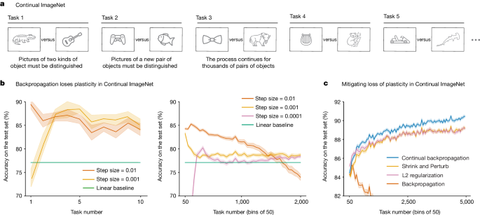
separate set of test images from the same classes. To adapt ImageNet to continual learning while minimizing all other changes, we constructed a sequence of binary classification tasks by

taking the classes in pairs. For example, the first task might be to distinguish cats from houses and the second might be to distinguish stop signs from school buses. With the 1,000 classes

in our dataset, we were able to form half a million binary classification tasks in this way. For each task, a deep-learning network was first trained on a subset of the images for the two

classes and then its performance was measured on a separate test set for the classes. After training and testing on one task, the next task began with a different pair of classes. We call

this problem ‘Continual ImageNet’. In Continual ImageNet, the difficulty of tasks remains the same over time. A drop in performance would mean the network is losing its learning ability, a

direct demonstration of loss of plasticity. We applied a wide variety of standard deep-learning networks to Continual ImageNet and tested many learning algorithms and parameter settings. To

assess the performance of the network on a task, we measured the percentage of test images that were correctly classified. The results shown in Fig. 1b are representative; they are for a

feed-forward convolutional network and for a training procedure, using unmodified backpropagation, that performed well on this problem in the first few tasks. Although these networks learned

up to 88% correct on the test set of the early tasks (Fig. 1b, left panel), by the 2,000th task, they had lost substantial plasticity for all values of the step-size parameter (right

panel). Some step sizes performed well on the first two tasks but then much worse on subsequent tasks, eventually reaching a performance level below that of a linear network. For other step

sizes, performance rose initially and then fell and was only slightly better than the linear network after 2,000 tasks. We found this to be a common pattern in our experiments: for a

well-tuned network, performance first improves and then falls substantially, ending near or below the linear baseline. We have observed this pattern for many network architectures, parameter

choices and optimizers. The specific choice of network architecture, algorithm parameters and optimizers affected when the performance started to drop, but a severe performance drop

occurred for a wide range of choices. The failure of standard deep-learning methods to learn better than a linear network in later tasks is direct evidence that these methods do not work

well in continual-learning problems. Algorithms that explicitly keep the weights of the network small were an exception to the pattern of failure and were often able to maintain plasticity

and even improve their performance over many tasks, as shown in Fig. 1c. L2 regularization adds a penalty for large weights; augmenting backpropagation with this enabled the network to

continue improving its learning performance over at least 5,000 tasks. The Shrink and Perturb algorithm11, which includes L2 regularization, also performed well. Best of all was our

continual backpropagation algorithm, which we discuss later. For all algorithms, we tested a wide range of parameter settings and performed many independent runs for statistical

significance. The presented curves are the best representative of each algorithm. For a second demonstration, we chose to use residual networks, class-incremental continual learning and the

CIFAR-100 dataset. Residual networks include layer-skipping connections as well as the usual layer-to-layer connections of conventional convolutional networks. The residual networks of today

are more widely used and produce better results than strictly layered networks38. Class-incremental continual learning39 involves sequentially adding new classes while testing on all

classes seen so far. In our demonstration, we started with training on five classes and then successively added more, five at a time, until all 100 were available. After each addition, the

networks were trained and performance was measured on all available classes. We continued training on the old classes (unlike in most work in class-incremental learning) to focus on

plasticity rather than on forgetting. In this demonstration, we used an 18-layer residual network with a variable number of heads, adding heads as new classes were added. We also used

further deep-learning techniques, including batch normalization, data augmentation, L2 regularization and learning-rate scheduling. These techniques are standardly used with residual

networks and are necessary for good performance. We call this our base deep-learning system. As more classes are added, correctly classifying images becomes more difficult and classification

accuracy would decrease even if the network maintained its ability to learn. To factor out this effect, we compare the accuracy of our incrementally trained networks with networks that were

retrained from scratch on the same subset of classes. For example, the network that was trained first on five classes, and then on all ten classes, is compared with a network retrained from

scratch on all ten classes. If the incrementally trained network performs better than a network retrained from scratch, then there is a benefit owing to training on previous classes, and if

it performs worse, then there is genuine loss of plasticity. The red line in Fig. 2b shows that incremental training was initially better than retraining, but after 40 classes, the

incrementally trained network showed loss of plasticity that became increasingly severe. By the end, when all 100 classes were available, the accuracy of the incrementally trained base

system was 5% lower than the retrained network (a performance drop equivalent to that of removing a notable algorithmic advance, such as batch normalization). Loss of plasticity was less

severe when Shrink and Perturb was added to the learning algorithm (in the incrementally trained network) and was eliminated altogether when continual backpropagation (see the ‘Maintaining

plasticity through variability and selective preservation’ section) was added. These additions also prevented units of the network from becoming inactive or redundant, as shown in Fig. 2c,d.

This demonstration involved larger networks and required more computation, but still we were able to perform extensive systematic tests. We found a robust pattern in the results that was

similar to what we found in ImageNet. In both cases, deep-learning networks exhibited substantial loss of plasticity. Altogether, these results, along with other extensive results in

Methods, constitute substantial evidence of plasticity loss. PLASTICITY LOSS IN REINFORCEMENT LEARNING Continual learning is essential to reinforcement learning in ways that go beyond its 

importance in supervised learning. Not only can the environment change but the behaviour of the learning agent can also change, thereby influencing the data it receives even if the

environment is stationary. For this reason, the need for continual learning is often more apparent in reinforcement learning, and reinforcement learning is an important setting in which to

demonstrate the tendency of deep learning towards loss of plasticity. Nevertheless, it is challenging to demonstrate plasticity loss in reinforcement learning in a systematic and rigorous

way. In part, this is because of the great variety of algorithms and experimental settings that are commonly used in reinforcement-learning research. Algorithms may learn value functions,

behaviours or both simultaneously and may involve replay buffers, world models and learned latent states. Experiments may be episodic, continuing or offline. All of these choices involve

several embedded choices of parameters. More fundamentally, reinforcement-learning algorithms affect the data seen by the agent. The learning ability of an algorithm is thus confounded with

its ability to generate informative data. Finally, and in part because of the preceding, reinforcement-learning results tend to be more stochastic and more widely varying than in supervised

learning. Altogether, demonstration of reinforcement-learning abilities, particularly negative results, tends to require more runs and generally much more experimental work and thus

inevitably cannot be as definitive as in supervised learning. Our first demonstration involves a reinforcement-learning algorithm applied to a simulated ant-like robot tasked with moving

forwards as rapidly and efficiently as possible. The agent–environment interaction comprises a series of episodes, each beginning in a standard state and lasting up to 1,000 time steps. On

each time step, the agent receives a reward depending on the forward distance travelled and the magnitude of its action (see Methods for details). An episode terminates in fewer than 1,000

steps if the ant jumps too high instead of moving forwards, as often happens early in learning. In the results to follow, we use the cumulative reward during an episode as our primary

performance measure. To make the task non-stationary (and thereby emphasize plasticity), the coefficient of friction between the feet of the ant and the floor is changed after every 2 

million time steps (but only at an episode boundary; details in Methods). For fastest walking, the agent must adapt (relearn) its way of walking each time the friction changes. For this

experiment, we used the proximal policy optimization (PPO) algorithm40. PPO is a standard deep reinforcement-learning algorithm based on backpropagation. It is widely used, for example, in

robotics9, in playing real-time strategy games41 and in aligning large language models from human feedback42. PPO performed well (see the red line in Fig. 3c) for the first 2 million steps,

up until the first change in friction, but then performed worse and worse. Note how the performance of the other algorithms in Fig. 3c decreased each time the friction changed and then

recovered as the agent adapted to the new friction, giving the plot a sawtooth appearance. PPO augmented with a specially tuned Adam optimizer24,43 performed much better (orange line in Fig.

3c) but still performed much worse over successive changes after the first two, indicating substantial loss of plasticity. On the other hand, PPO augmented with L2 regularization and

continual backpropagation largely maintained their plasticity as the problem changed. Now consider the same ant-locomotion task except with the coefficient of friction held constant at an

intermediate value over 50 million time steps. The red line in Fig. 4a shows that the average performance of PPO increased for about 3 million steps but then collapsed. After 20 million

steps, the ant is failing every episode and is unable to learn to move forwards efficiently. The red lines in the other panels of Fig. 4 provide further insight into the loss of plasticity

of PPO. They suggest that the network may be losing plasticity in the same way as in our supervised learning results (see Fig. 2 and Extended Data Fig. 3c). In both cases, most of the

network’s units became dormant during the experiment, and the network markedly lost stable rank. The addition of L2 regularization mitigated the performance degradation by preventing

continual growth of weights but also resulted in very small weights (Fig. 4d), which prevented the agent from committing to good behaviour. The addition of continual backpropagation

performed better overall. We present results for continual backpropagation only with (slight) L2 regularization, because without it, performance was highly sensitive to parameter settings.

These results show that plasticity loss can be catastrophic in both deep reinforcement learning as well as deep supervised learning. MAINTAINING PLASTICITY Surprisingly, popular methods such

as Adam, Dropout and normalization actually increased loss of plasticity (see Extended Data Fig. 4a). L2 regularization, on the other hand, reduced loss of plasticity in many cases (purple

line in Figs. 1, 3 and 4). L2 regularization stops the weights from becoming too large by moving them towards zero at each step. The small weights allow the network to remain plastic.

Another existing method that reduced loss of plasticity is Shrink and Perturb11 (orange line in Figs. 1 and 2). Shrink and Perturb is L2 regularization plus small random changes in weights

at each step. The injection of variability into the network can reduce dormancy and increase the diversity of the representation (Figs. 2 and 4). Our results indicate that non-growing

weights and sustained variability in the network may be important for maintaining plasticity. We now describe a variation of the backpropagation algorithm that is explicitly designed to

inject variability into the network and keep some of its weights small. Conventional backpropagation has two main parts: initialization with small random weights before training and then

gradient descent at each training step. The initialization provides variability initially, but, as we have seen, with continued training, variability tends to be lost, as well as plasticity

along with it. To maintain the variability, our new algorithm, continual backpropagation, reinitializes a small number of units during training, typically fewer than one per step. To prevent

disruption of what the network has already learned, only the least-used units are considered for reinitialization. See Methods for details. The blue line in Fig. 1c shows the performance of

continual backpropagation on Continual ImageNet. It mitigated loss of plasticity in Continual ImageNet while outperforming existing methods. Similarly, the blue lines in Fig. 2 show the

performance of continual backpropagation on class-incremental CIFAR-100 and its effect on the evolution of dormant units and stable rank. Continual backpropagation fully overcame loss of

plasticity, with a high stable rank and almost no dead units throughout learning. In reinforcement learning, continual backpropagation was applied together with L2 regularization (a small

amount of regularization was added to prevent excessive sensitivity to parameters in reinforcement-learning experiments). The blue line in Fig. 3 shows the performance of PPO with continual

backpropagation on the ant-locomotion problem with changing friction. PPO with continual backpropagation performed much better than standard PPO, with little or no loss of plasticity. On the

ant-locomotion problem with constant friction (Fig. 4), PPO with continual backpropagation continued improving throughout the experiment. The blue lines in Fig. 4b–d show the evolution of

the correlates of loss of plasticity when we used continual backpropagation. PPO with continual backpropagation had few dormant units, a high stable rank and an almost constant average

weight magnitude. Our results are consistent with the idea that small weights reduce loss of plasticity and that a continual injection of variability further mitigates loss of plasticity.

Although Shrink and Perturb adds variability to all weights, continual backpropagation does so selectively, and this seems to enable it to better maintain plasticity. Continual

backpropagation involves a form of variation and selection in the space of neuron-like units, combined with continuing gradient descent. The variation and selection is reminiscent of

trial-and-error processes in evolution and behaviour44,45,46,47 and has precursors in many earlier ideas, including Keifer–Wolfowitz methods48 and restart methods49 in engineering and

feature-search methods in machine learning31,32,33,34,35,50. Continual backpropagation brings a form of this old idea to modern deep learning. However, it is just one variation of this idea;

other variations are possible and some of these have been explored in recent work25,27. We look forward to future work that explicitly compares and further refines these variations.

DISCUSSION Deep learning is an effective and valuable technology in settings in which learning occurs in a special training phase and not thereafter. In settings in which learning must

continue, however, we have shown that deep learning does not work. By deep learning, we mean the existing standard algorithms for learning in multilayer artificial neural networks and by not

work, we mean that, over time, they fail to learn appreciably better than shallow networks. We have shown such loss of plasticity using supervised-learning datasets and

reinforcement-learning tasks on which deep learning has previously excelled and for a wide range of networks and standard learning algorithms. Taking a closer look, we found that, during

training, many of the networks’ neuron-like units become dormant, overcommitted and similar to each other, hampering the ability of the networks to learn new things. As they learn, standard

deep-learning networks gradually and irreversibly lose their diversity and thus their ability to continue learning. Plasticity loss is often severe when learning continues for many tasks,

but may not occur at all for small numbers of tasks. The problem of plasticity loss is not intrinsic to deep learning. Deep artificial neural networks trained by gradient descent are

perfectly capable of maintaining their plasticity, apparently indefinitely, as we have shown with the Shrink and Perturb algorithm and particularly with the new continual backpropagation

algorithm. Both of these algorithms extend standard deep learning by adding a source of continuing variability to the weights of the network, and continual backpropagation restricts this

variability to the units of the network that are at present least used, minimizing damage to the operation of the network. That is, continual backpropagation involves a form of variation and

selection in the space of neuron-like units, combined with continuing gradient descent. This idea has many historical antecedents and will probably require further development to reach its

most effective form. METHODS SPECIFICS OF CONTINUAL BACKPROPAGATION Continual backpropagation selectively reinitializes low-utility units in the network. Our utility measure, called the

contribution utility, is defined for each connection or weight and each unit. The basic intuition behind the contribution utility is that the magnitude of the product of units’ activation

and outgoing weight gives information about how valuable this connection is to its consumers. If the contribution of a hidden unit to its consumer is small, its contribution can be

overwhelmed by contributions from other hidden units. In such a case, the hidden unit is not useful to its consumer. We define the contribution utility of a hidden unit as the sum of the

utilities of all its outgoing connections. The contribution utility is measured as a running average of instantaneous contributions with a decay rate, _η_, which is set to 0.99 in all

experiments. In a feed-forward neural network, the contribution utility, U_l_[_i_], of the _i_th hidden unit in layer _l_ at time _t_ is updated as $${{\bf{u}}}_{l}[i]=\eta \times

{{\bf{u}}}_{l}[i]+(1-\eta )\times | {{\bf{h}}}_{l,i,t}| \times \mathop{\sum }\limits_{k=1}^{{n}_{l+1}}| {{\bf{w}}}_{l,i,k,t}| ,$$ (1) in which H_l_,_i_,_t_ is the output of the _i_th hidden

unit in layer _l_ at time _t_, W_l_,_i_,_k_,_t_ is the weight connecting the _i_th unit in layer _l_ to the _k_th unit in layer _l_ + 1 at time _t_ and _n__l_+1 is the number of units in

layer _l_ + 1. When a hidden unit is reinitialized, its outgoing weights are initialized to zero. Initializing the outgoing weights as zero ensures that the newly added hidden units do not

affect the already learned function. However, initializing the outgoing weight to zero makes the new unit vulnerable to immediate reinitialization, as it has zero utility. To protect new

units from immediate reinitialization, they are protected from a reinitialization for maturity threshold _m_ number of updates. We call a unit mature if its age is more than _m_. Every step,

a fraction of mature units _ρ_, called the replacement rate, is reinitialized in every layer. The replacement rate _ρ_ is typically set to a very small value, meaning that only one unit is

replaced after hundreds of updates. For example, in class-incremental CIFAR-100 (Fig. 2) we used continual backpropagation with a replacement rate of 10−5. The last layer of the network in

that problem had 512 units. At each step, roughly 512 × 10−5 = 0.00512 units are replaced. This corresponds to roughly one replacement after every 1/0.00512 ≈ 200 updates or one replacement

after every eight epochs on the first five classes. The final algorithm combines conventional backpropagation with selective reinitialization to continually inject random units from the

initial distribution. Continual backpropagation performs a gradient descent and selective reinitialization step at each update. Algorithm 1 specifies continual backpropagation for a

feed-forward neural network. In cases in which the learning system uses mini-batches, the instantaneous contribution utility can be used by averaging the utility over the mini-batch instead

of keeping a running average to save computation (see Extended Data Fig. 5d for an example). Continual backpropagation overcomes the limitation of previous work34,35 on selective

reinitialization and makes it compatible with modern deep learning. ALGORITHM 1 CONTINUAL BACKPROPAGATION FOR A FEED-FORWARD NETWORK WITH _L_ LAYERS Set replacement rate _ρ_, decay rate _η_

and maturity threshold _m_ Initialize the weights W0,…, W_L_−1, in which W_l_ is sampled from distribution _d__l_ Initialize utilities U1,…, U_L_−1, number of units to replace _c_1,…, 

_c__L_−1, and ages A1,…, A_L_−1 to 0 FOR each input X_t_ DO Forward pass: pass X_t_ through the network to get the prediction \(\widehat{{{\bf{y}}}_{t}}\) Evaluate: receive loss

\(l({{\bf{x}}}_{t},\widehat{{{\bf{y}}}_{t}})\) Backward pass: update the weights using SGD or one of its variants FOR layer _l_ in 1: _L_ − 1 DO Update age: A_l_ = A_l_ + 1 Update unit

utility: see equation (1) Find eligible units: _n_eligible = number of units with age greater than _m_ Update number of units to replace: _c__l_ = _c__l_ + _n_eligible × _ρ_ IF _c__l_ > 1

Find the unit with smallest utility and record its index as _r_ Reinitialize input weights: resample W_l_−1[:,_r_] from distribution _d__l_ Reinitialize output weights: set W_l_[_r_,:] to 0

Reinitialize utility and age: set U_l_[_r_] = 0 and A_l_[_r_] = 0 Update number of units to replace: _c__l_ = _c__l_ − 1 END FOR END FOR DETAILS OF CONTINUAL IMAGENET The ImageNet database

we used consists of 1,000 classes, each of 700 images. The 700 images for each class were divided into 600 images for a training set and 100 images for a test set. On each binary

classification task, the deep-learning network was first trained on the training set of 1,200 images and then its classification accuracy was measured on the test set of 200 images. The

training consisted of several passes through the training set, called epochs. For each task, all learning algorithms performed 250 passes through the training set using mini-batches of size

100. All tasks used the downsampled 32 × 32 version of the ImageNet dataset, as is often done to save computation51. All algorithms on Continual ImageNet used a convolutional network. The

network had three convolutional-plus-max-pooling layers, followed by three fully connected layers, as detailed in Extended Data Table 3. The final layer consisted of just two units, the

heads, corresponding to the two classes. At task changes, the input weights of the heads were reset to zero. Resetting the heads in this way can be viewed as introducing new heads for the

new tasks. This resetting of the output weights is not ideal for studying plasticity, as the learning system gets access to privileged information on the timing of task changes (and we do

not use it in other experiments in this paper). We use it here because it is the standard practice in deep continual learning for this type of problem in which the learning system has to

learn a sequence of independent tasks52. In this problem, we reset the head of the network at the beginning of each task. It means that, for a linear network, the whole network is reset.

That is why the performance of a linear network will not degrade in Continual ImageNet. As the linear network is a baseline, having a low-variance estimate of its performance is desirable.

The value of this baseline is obtained by averaging over thousands of tasks. This averaging gives us a much better estimate of its performance than other networks. The network was trained

using SGD with momentum on the cross-entropy loss and initialized once before the first task. The momentum hyperparameter was 0.9. We tested various step-size parameters for backpropagation

but only presented the performance for step sizes 0.01, 0.001 and 0.0001 for clarity of Fig. 1b. We performed 30 runs for each hyperparameter value, varying the sequence of tasks and other

randomness. Across different hyperparameters and algorithms, the same sequences of pairs of classes were used. We now describe the hyperparameter selection for L2 regularization, Shrink and

Perturb and continual backpropagation. The main text presents the results for these algorithms on Continual ImageNet in Fig. 1c. We performed a grid search for all algorithms to find the set

of hyperparameters that had the highest average classification accuracy over 5,000 tasks. The values of hyperparameters used for the grid search are described in Extended Data Table 2. L2

regularization has two hyperparameters, step size and weight decay. Shrink and Perturb has three hyperparameters, step size, weight decay and noise variance. We swept over two

hyperparameters of continual backpropagation: step size and replacement rate. The maturity threshold in continual backpropagation was set to 100. For both backpropagation and L2

regularization, the performance was poor for step sizes of 0.1 or 0.003. We chose to only use step sizes of 0.03 and 0.01 for continual backpropagation and Shrink and Perturb. We performed

ten independent runs for all sets of hyperparameters. Then we performed another 20 runs to complete 30 runs for the best-performing set of hyperparameters to produce the results in Fig. 1c.

CLASS-INCREMENTAL CIFAR-100 In the class-incremental CIFAR-100, the learning system gets access to more and more classes over time. Classes are provided to the learning system in increments

of five. First, it has access to just five classes, then ten and so on, until it gets access to all 100 classes. The learning system is evaluated on the basis of how well it can discriminate

between all the available classes at present. The dataset consists of 100 classes with 600 images each. The 600 images for each class were divided into 450 images to create a training set,

50 for a validation set and 100 for a test set. Note that the network is trained on all data from all classes available at present. First, it is trained on data from just five classes, then

from all ten classes and so on, until finally, it is trained from data from all 100 classes simultaneously. After each increment, the network was trained for 200 epochs, for a total of 4,000

epochs for all 20 increments. We used a learning-rate schedule that resets at the start of each increment. For the first 60 epochs of each increment, the learning rate was set to 0.1, then

to 0.02 for the next 60 epochs, then 0.004 for the next 40 epochs and to 0.0008 for the last 40 epochs; we used the initial learning rate and learning-rate schedule reported in ref. 53.

During the 200 epochs of training for each increment, we kept track of the network with the best accuracy on the validation set. To prevent overfitting, at the start of each new increment,

we reset the weights of the network to the weights of the best-performing (on the validation set) network found during the previous increment; this is equivalent to early stopping for each

different increment. We used an 18-layer deep residual network38 for all experiments on class-incremental CIFAR-100. The network architecture is described in detail in Extended Data Table 1.

The weights of convolutional and linear layers were initialized using Kaiming initialization54, the weights for the batch-norm layers were initialized to one and all of the bias terms in

the network were initialized to zero. Each time five new classes were made available to the network, five more output units were added to the final layer of the network. The weights and

biases of these output units were initialized using the same initialization scheme. The weights of the network were optimized using SGD with a momentum of 0.9, a weight decay of 0.0005 and a

mini-batch size of 90. We used several steps of data preprocessing before the images were presented to the network. First, the value of all the pixels in each image was rescaled between 0

and 1 through division by 255. Then, each pixel in each channel was centred and rescaled by the average and standard deviation of the pixel values of each channel, respectively. Finally, we

applied three random data transformations to each image before feeding it to the network: randomly horizontally flip the image with a probability of 0.5, randomly crop the image by padding

the image with 4 pixels on each side and randomly cropping to the original size, and randomly rotate the image between 0 and 15°. The first two steps of preprocessing were applied to the

training, validation and test sets, but the random transformations were only applied to the images in the training set. We tested several hyperparameters to ensure the best performance for

each different algorithm with our specific architecture. For the base system, we tested values for the weight decay parameter in {0.005, 0.0005, 0.00005}. A weight-decay value of 0.0005

resulted in the best performance in terms of area under the curve for accuracy on the test set over the 20 increments. For Shrink and Perturb, we used the weight-decay value of the base

system and tested values for the standard deviation of the Gaussian noise in {10−4, 10−5, 10−6}; 10−5 resulted in the best performance. For continual backpropagation, we tested values for

the maturity threshold in {1,000, 10,000} and for the replacement rate in {10−4, 10−5, 10−6} using the contribution utility described in equation (1). A maturity threshold of 1,000 and a

replacement rate of 10−5 resulted in the best performance. Finally, for the head-resetting baseline, in Extended Data Fig. 1a, we used the same hyperparameters as for the base system, but

the output layer was reinitialized at the start of each increment. In Fig. 2d, we plot the stable rank of the representation in the penultimate layer of the network and the percentage of

dead units in the full network. For a matrix \({\boldsymbol{\Phi }}\in {{\mathbb{R}}}^{n\times m}\) with singular values _σ__k_ sorted in descending order for _k_ = 1, 2,…, _q_ and _q_ = 

max(_n_, _m_), the stable rank55 is \(\min \left\{k:\frac{{\Sigma }_{i}^{k}{\sigma }_{i}}{{\Sigma }_{j}^{q}{\sigma }_{j}} > 0.99\right\}\). For reference, we also implemented a network

with the same hyperparameters as the base system but that was reinitialized at the beginning of each increment. Figure 2b shows the performance of each algorithm relative to the performance

of the reinitialized network. For completeness, Extended Data Fig. 1a shows the test accuracy of each algorithm in each different increment. The final accuracy of continual backpropagation

on all 100 classes was 76.13%, whereas Extended Data Fig. 1b shows the performance of continual backpropagation for different replacement rates with a maturity threshold of 1,000. For all

algorithms that we tested, there was no correlation between when a class was presented and the accuracy of that class, implying that the temporal order of classes did not affect performance.

ROBUST LOSS OF PLASTICITY IN PERMUTED MNIST We now use a computationally cheap problem based on the MNIST dataset56 to test the generality of loss of plasticity across various conditions.

MNIST is one of the most common supervised-learning datasets used in deep learning. It consists of 60,000, 28 × 28, greyscale images of handwritten digits from 0 to 9, together with their

correct labels. For example, the left image in Extended Data Fig. 3a shows an image that is labelled by the digit 7. The smaller number of classes and the simpler images enable much smaller

networks to perform well on this dataset than are needed on ImageNet or CIFAR-100. The smaller networks in turn mean that much less computation is needed to perform the experiments and thus

experiments can be performed in greater quantities and under a variety of different conditions, enabling us to perform deeper and more extensive studies of plasticity. We created a continual

supervised-learning problem using permuted MNIST datasets57,58. An individual permuted MNIST dataset is created by permuting the pixels in the original MNIST dataset. The right image in

Extended Data Fig. 3a is an example of such a permuted image. Given a way of permuting, all 60,000 images are permuted in the same way to produce the new permuted MNIST dataset. Furthermore,

we normalized pixel values between 0 and 1 by dividing by 255. By repeatedly randomly selecting from the approximately 101930 possible permutations, we created a sequence of 800 permuted

MNIST datasets and supervised-learning tasks. For each task, we presented each of its 60,000 images one by one in random order to the learning network. Then we moved to the next permuted

MNIST task and repeated the whole procedure, and so on for up to 800 tasks. No indication was given to the network at the time of task switching. With the pixels being permuted in a

completely unrelated way, we might expect classification performance to fall substantially at the time of each task switch. Nevertheless, across tasks, there could be some savings, some

improvement in speed of learning or, alternatively, there could be loss of plasticity—loss of the ability to learn across tasks. The network was trained on a single pass through the data and

there were no mini-batches. We call this problem Online Permuted MNIST. We applied feed-forward neural networks with three hidden layers to Online Permuted MNIST. We did not use

convolutional layers, as they could not be helpful on the permuted problem because the spatial information is lost; in MNIST, convolutional layers are often not used even on the standard,

non-permuted problem. For each example, the network estimated the probabilities of each of the tem classes, compared them to the correct label and performed SGD on the cross-entropy loss. As

a measure of online performance, we recorded the percentage of times the network correctly classified each of the 60,000 images in the task. We plot this per-task performance measure versus

task number in Extended Data Fig. 3b. The weights were initialized according to a Kaiming distribution. The left panel of Extended Data Fig. 3b shows the progression of online performance

across tasks for a network with 2,000 units per layer and various values of the step-size parameter. Note that that performance first increased across tasks, then began falling steadily

across all subsequent tasks. This drop in performance means that the network is slowly losing the ability to learn from new tasks. This loss of plasticity is consistent with the loss of

plasticity that we observed in ImageNet and CIFAR-100. Next, we varied the network size. Instead of 2,000 units per layer, we tried 100, 1,000 and 10,000 units per layer. We ran this

experiment for only 150 tasks, primarily because the largest network took much longer to run. The performances at good step sizes for each network size are shown in the middle panel of

Extended Data Fig. 3b. Loss of plasticity with continued training is most pronounced at the smaller network sizes, but even the largest networks show some loss of plasticity. Next, we

studied the effect of the rate at which the task changed. Going back to the original network with 2,000-unit layers, instead of changing the permutation after each 60,000 examples, we now

changed it after each 10,000, 100,000 or 1 million examples and ran for 48 million examples in total no matter how often the task changed. The examples in these cases were selected randomly

with replacement for each task. As a performance measure of the network on a task, we used the percentage correct over all of the images in the task. The progression of performance is shown

in the right panel in Extended Data Fig. 3b. Again, performance fell across tasks, even if the change was very infrequent. Altogether, these results show that the phenomenon of loss of

plasticity robustly arises in this form of backpropagation. Loss of plasticity happens for a wide range of step sizes, rates of distribution change and for both underparameterized and

overparameterized networks. LOSS OF PLASTICITY WITH DIFFERENT ACTIVATIONS IN THE SLOWLY-CHANGING REGRESSION PROBLEM There remains the issue of the network’s activation function. In our

experiments so far, we have used ReLU, the most popular choice at present, but there are several other possibilities. For these experiments, we switched to an even smaller, more idealized

problem. Slowly-Changing Regression is a computationally inexpensive problem in which we can run a single experiment on a CPU core in 15 min, allowing us to perform extensive studies. As its

name suggests, this problem is a regression problem—meaning that the labels are real numbers, with a squared loss, rather than nominal values with a cross-entropy loss—and the

non-stationarity is slow and continual rather than abrupt, as in a switch from one task to another. In Slowly-Changing Regression, we study loss of plasticity for networks with six popular

activation functions: sigmoid, tanh, ELU59, leaky ReLU60, ReLU61 and Swish62. In Slowly-Changing Regression, the learner receives a sequence of examples. The input for each example is a

binary vector of size _m_ + 1. The input has _f_ slow-changing bits, _m_ − _f_ random bits and then one constant bit. The first _f_ bits in the input vector change slowly. After every _T_

examples, one of the first _f_ bits is chosen uniformly at random and its value is flipped. These first _f_ bits remain fixed for the next _T_ examples. The parameter _T_ allows us to

control the rate at which the input distribution changes. The next _m_ − _f_ bits are randomly sampled for each example. Last, the (_m_ + 1)th bit is a bias term with a constant value of

one. The target output is generated by running the input vector through a neural network, which is set at the start of the experiment and kept fixed. As this network generates the target

output and represents the desired solution, we call it the target network. The weights of the target networks are randomly chosen to be +1 or −1. The target network has one hidden layer with

the linear threshold unit (LTU) activation. The value of the _i_th LTU is one if the input is above a threshold _θ__i_ and 0 otherwise. The threshold _θ__i_ is set to be equal to (_m_ + 1) 

× _β_ − _S__i_, in which _β_ ∈ [0, 1] and _S__i_ is the number of input weights with negative value63. The details of the input and target function in the Slowly-Changing Regression problem

are also described in Extended Data Fig. 2a. The details of the specific instance of the Slowly-Changing Regression problem we use in this paper and the learning network used to predict its

output are listed in Extended Data Table 4. Note that the target network is more complex than the learning network, as the target network is wider, with 100 hidden units, whereas the learner

has just five hidden units. Thus, because the input distribution changes every _T_ example and the target function is more complex than what the learner can represent, there is a need to

track the best approximation. We applied learning networks with different activation functions to the Slowly-Changing Regression. The learner used the backpropagation algorithm to learn the

weights of the network. We used a uniform Kaiming distribution54 to initialize the weights of the learning network. The distribution is _U_(−_b_, _b_) with bound,

\(b={\rm{g}}{\rm{a}}{\rm{i}}{\rm{n}}\times \sqrt{\frac{3}{{\rm{n}}{\rm{u}}{\rm{m}}{\rm{\_}}{\rm{i}}{\rm{n}}{\rm{p}}{\rm{u}}{\rm{t}}{\rm{s}}}}\), in which gain is chosen such that the

magnitude of inputs does not change across layers. For tanh, sigmoid, ReLU and leaky ReLU, the gain is 5/3, 1, \(\sqrt{2}\) and \(\sqrt{2/(1+{\alpha }^{2})}\), respectively. For ELU and

Swish, we used \({\rm{gain}}=\sqrt{2}\), as was done in the original papers59,62. We ran the experiment on the Slowly-Changing Regression problem for 3 million examples. For each activation

and value of step size, we performed 100 independent runs. First, we generated 100 sequences of examples (input–output pairs) for the 100 runs. Then these 100 sequences of examples were used

for experiments with all activations and values of the step-size parameter. We used the same sequence of examples to control the randomness in the data stream across activations and step

sizes. The results of the experiments are shown in Extended Data Fig. 2b. We measured the squared error, that is, the square of the difference between the true target and the prediction made

by the learning network. In Extended Data Fig. 2b, the squared error is presented in bins of 40,000 examples. This means that the first data point is the average squared error on the first

40,000 examples, the next is the average squared error on the next 40,000 examples and so on. The shaded region in the figure shows the standard error of the binned error. Extended Data Fig.

2b shows that, in Slowly-Changing Regression, after performing well initially, the error increases for all step sizes and activations. For some activations such as ReLU and tanh, loss of

plasticity is severe, and the error increases to the level of the linear baseline. Although for other activations such as ELU loss of plasticity is less severe, there is still a notable loss

of plasticity. These results mean that loss of plasticity is not resolved by using commonly used activations. The results in this section complement the results in the rest of the article

and add to the generality of loss of plasticity in deep learning. UNDERSTANDING LOSS OF PLASTICITY We now turn our attention to understanding why backpropagation loses plasticity in

continual-learning problems. The only difference in the learner over time is the network weights. In the beginning, the weights were small random numbers, as they were sampled from the

initial distribution; however, after learning some tasks, the weights became optimized for the most recent task. Thus, the starting weights for the next task are qualitatively different from

those for the first task. As this difference in the weights is the only difference in the learning algorithm over time, the initial weight distribution must have some unique properties that

make backpropagation plastic in the beginning. The initial random distribution might have many properties that enable plasticity, such as the diversity of units, non-saturated units, small

weight magnitude etc. As we now demonstrate, many advantages of the initial distribution are lost concurrently with loss of plasticity. The loss of each of these advantages partially

explains the degradation in performance that we have observed. We then provide arguments for how the loss of these advantages could contribute to loss of plasticity and measures that

quantify the prevalence of each phenomenon. We provide an in-depth study of the Online Permuted MNIST problem that will serve as motivation for several solution methods that could mitigate

loss of plasticity. The first noticeable phenomenon that occurs concurrently with the loss of plasticity is the continual increase in the fraction of constant units. When a unit becomes

constant, the gradients flowing back from the unit become zero or very close to zero. Zero gradients mean that the weights coming into the unit do not change, which means that this unit

loses all of its plasticity. In the case of ReLU activations, this occurs when the output of the activations is zero for all examples of the task; such units are often said to be dead64,65.

In the case of the sigmoidal activation functions, this phenomenon occurs when the output of a unit is too close to either of the extreme values of the activation function; such units are

often said to be saturated66,67. To measure the number of dead units in a network with ReLU activation, we count the number of units with a value of zero for all examples in a random sample

of 2,000 images at the beginning of each new task. An analogous measure in the case of sigmoidal activations is the number of units that are _ϵ_ away from either of the extreme values of the

function for some small positive _ϵ_ (ref. 68). We only focus on ReLU networks in this section. In our experiments on the Online Permuted MNIST problem, the deterioration of online

performance is accompanied by a large increase in the number of dead units (left panel of Extended Data Fig. 3c). For the step size of 0.01, up to 25% of units die after 800 tasks. In the

permuted MNIST problem, in which all inputs are positive because they are normalized between 0 and 1, once a unit in the first layer dies, it stays dead forever. Thus, an increase in dead

units directly decreases the total capacity of the network. In the next section, we will see that methods that stop the units from dying can substantially reduce loss of plasticity. This

further supports the idea that the increase in dead units is one of the causes of loss of plasticity in backpropagation. Another phenomenon that occurs with loss of plasticity is the steady

growth of the network’s average weight magnitude. We measure the average magnitude of the weights by adding up their absolute values and dividing by the total number of weights in the

network. In the permuted MNIST experiment, the degradation of online classification accuracy of backpropagation observed in Extended Data Fig. 3b is associated with an increase in the

average magnitude of the weights (centre panel of Extended Data Fig. 3c). The growth of the magnitude of the weights of the network can represent a problem because large weight magnitudes

are often associated with slower learning. The weights of a neural network are directly linked to the condition number of the Hessian matrix in the second-order Taylor approximation of the

loss function. The condition number of the Hessian is known to affect the speed of convergence of SGD algorithms (see ref. 69 for an illustration of this phenomenon in convex optimization).

Consequently, the growth in the magnitude of the weights could lead to an ill-conditioned Hessian matrix, resulting in a slower convergence. The last phenomenon that occurs with the loss of

plasticity is the drop in the effective rank of the representation. Similar to the rank of a matrix, which represents the number of linearly independent dimensions, the effective rank takes

into consideration how each dimension influences the transformation induced by a matrix70. A high effective rank indicates that most of the dimensions of the matrix contribute similarly to

the transformation induced by the matrix. On the other hand, a low effective rank corresponds to most dimensions having no notable effect on the transformation, implying that the information

in most of the dimensions is close to being redundant. Formally, consider a matrix \(\Phi \in {{\mathbb{R}}}^{n\times m}\) with singular values _σ__k_ for _k_ = 1, 2,…, _q_, and _q_ = 

max(_n_, _m_). Let _p__k_ = _σ__k_/∥Σ∥1, in which Σ is the vector containing all the singular values and ∥⋅∥1 is the _ℓ_1 norm. The effective rank of matrix Φ, or erank(Φ), is defined as

$$\begin{array}{l}{\rm{e}}{\rm{r}}{\rm{a}}{\rm{n}}{\rm{k}}({\boldsymbol{\Phi }})\dot{=}\exp \{H({p}_{1},{p}_{2},...,{p}_{q})\},\\ {\rm{in\;

which}}\,H({p}_{1},{p}_{2},...,{p}_{q})=-\mathop{\sum }\limits_{k=1}^{q}{p}_{k}\log ({p}_{k}).\end{array}$$ (2) Note that the effective rank is a continuous measure that ranges between one

and the rank of matrix Φ. In the case of neural networks, the effective rank of a hidden layer measures the number of units that can produce the output of the layer. If a hidden layer has a

low effective rank, then a small number of units can produce the output of the layer, meaning that many of the units in the hidden layer are not providing any useful information. We

approximate the effective rank on a random sample of 2,000 examples before training on each task. In our experiments, loss of plasticity is accompanied by a decrease in the average effective

rank of the network (right panel of Extended Data Fig. 3c). This phenomenon in itself is not necessarily a problem. After all, it has been shown that gradient-based optimization seems to

favour low-rank solutions through implicit regularization of the loss function or implicit minimization of the rank itself71,72. However, a low-rank solution might be a bad starting point

for learning from new observations because most of the hidden units provide little to no information. The decrease in effective rank could explain the loss of plasticity in our experiments

in the following way. After each task, the learning algorithm finds a low-rank solution for the current task, which then serves as the initialization for the next task. As the process

continues, the effective rank of the representation layer keeps decreasing after each task, limiting the number of solutions that the network can represent immediately at the start of each

new task. In this section, we looked deeper at the networks that lost plasticity in the Online Permuted MNIST problem. We noted that the only difference in the learning algorithm over time

is the weights of the network, which means that the initial weight distribution has some properties that allowed the learning algorithm to be plastic in the beginning. And as learning

progressed, the weights of the network moved away from the initial distribution and the algorithm started to lose plasticity. We found that loss of plasticity is correlated with an increase

in weight magnitude, a decrease in the effective rank of the representation and an increase in the fraction of dead units. Each of these correlates partially explains loss of plasticity

faced by backpropagation. EXISTING DEEP-LEARNING METHODS FOR MITIGATING LOSS OF PLASTICITY We now investigate several existing methods and test how they affect loss of plasticity. We study

five existing methods: L2 regularization73, Dropout74, online normalization75, Shrink and Perturb11 and Adam43. We chose L2 regularization, Dropout, normalization and Adam because these

methods are commonly used in deep-learning practice. Although Shrink and Perturb is not a commonly used method, we chose it because it reduces the failure of pretraining, a problem that is

an instance of loss of plasticity. To assess if these methods can mitigate loss of plasticity, we tested them on the Online Permuted MNIST problem using the same network architecture we used

in the previous section, ‘Understanding loss of plasticity’. Similar to the previous section, we measure the online classification accuracy on all 60,000 examples of the task. All the

algorithms used a step size of 0.003, which was the best-performing step size for backpropagation in the left panel of Extended Data Fig. 3b. We also use the three correlates of loss of

plasticity found in the previous section to get a deeper understanding of the performance of these methods. An intuitive way to address loss of plasticity is to use weight regularization, as

loss of plasticity is associated with a growth of weight magnitudes, shown in the previous section. We used L2 regularization, which adds a penalty to the loss function proportional to the

_ℓ_2 norm of the weights of the network. The L2 regularization penalty incentivizes SGD to find solutions that have a low weight magnitude. This introduces a hyperparameter _λ_ that

modulates the contribution of the penalty term. The purple line in the left panel of Extended Data Fig. 4a shows the performance of L2 regularization on the Online Permuted MNIST problem.

The purple lines in the other panels of Extended Data Fig. 4a show the evolution of the three correlates of loss of plasticity with L2 regularization. For L2 regularization, the weight

magnitude does not continually increase. Moreover, as expected, the non-increasing weight magnitude is associated with lower loss of plasticity. However, L2 regularization does not fully

mitigate loss of plasticity. The other two correlates for loss of plasticity explain this, as the percentage of dead units kept increasing and the effective rank kept decreasing. Finally,

Extended Data Fig. 4b shows the performance of L2 regularization for different values of _λ_. The regularization parameter _λ_ controlled the peak of the performance and how quickly it

decreased. A method related to weight regularization is Shrink and Perturb11. As the name suggests, Shrink and Perturb performs two operations; it shrinks all the weights and then adds

random Gaussian noise to these weights. The introduction of noise introduces another hyperparameter, the standard deviation of the noise. Owing to the shrinking part of Shrink and Perturb,

the algorithm favours solutions with smaller average weight magnitude than backpropagation. Moreover, the added noise prevents units from dying because it adds a non-zero probability that a

dead unit will become active again. If Shrink and Perturb mitigates these correlates to loss of plasticity, it could reduce loss of plasticity. The performance of Shrink and Perturb is shown

in orange in Extended Data Fig. 4. Similar to L2 regularization, Shrink and Perturb stops the weight magnitude from continually increasing. Moreover, it also reduces the percentage of dead

units. However, it has a lower effective rank than backpropagation, but still higher than that of L2 regularization. Not only does Shrink and Perturb have a lower loss of plasticity than

backpropagation but it almost completely mitigates loss of plasticity in Online Permuted MNIST. However, Shrink and Perturb was sensitive to the standard deviation of the noise. If the noise

was too high, loss of plasticity was much more severe, and if it was too low, it did not have any effect. An important technique in modern deep learning is called Dropout74. Dropout

randomly sets each hidden unit to zero with a small probability, which is a hyperparameter of the algorithm. The performance of Dropout is shown in pink in Extended Data Fig. 4. Dropout

showed similar measures of percentage of dead units, weight magnitude and effective rank as backpropagation, but, surprisingly, showed higher loss of plasticity. The poor performance of

Dropout is not explained by our three correlates of loss of plasticity, which means that there are other possible causes of loss of plasticity. A thorough investigation of Dropout is beyond

the scope of this paper, though it would be an interesting direction for future work. We found that a higher Dropout probability corresponded to a faster and sharper drop in performance.

Dropout with probability of 0.03 performed the best and its performance was almost identical to that of backpropagation. However, Extended Data Fig. 4a shows the performance for a Dropout

probability of 0.1 because it is more representative of the values used in practice. Another commonly used technique in deep learning is batch normalization76. In batch normalization, the

output of each hidden layer is normalized and rescaled using statistics computed from each mini-batch of data. We decided to include batch normalization in this investigation because it is a

popular technique often used in practice. Because batch normalization is not amenable to the online setting used in the Online Permuted MNIST problem, we used online normalization77

instead, an online variant of batch normalization. Online normalization introduces two hyperparameters used for the incremental estimation of the statistics in the normalization steps. The

performance of online normalization is shown in green in Extended Data Fig. 4. Online normalization had fewer dead units and a higher effective rank than backpropagation in the earlier

tasks, but both measures deteriorated over time. In the later tasks, the network trained using online normalization has a higher percentage of dead units and a lower effective rank than the

network trained using backpropagation. The online classification accuracy is consistent with these results. Initially, it has better classification accuracy, but later, its classification

accuracy becomes lower than that of backpropagation. For online normalization, the hyperparameters changed when the performance of the method peaked, and it also slightly changed how fast it

got to its peak performance. No assessment of alternative methods can be complete without Adam43, as it is considered one of the most useful tools in modern deep learning. The Adam

optimizer is a variant of SGD that uses an estimate of the first moment of the gradient scaled inversely by an estimate of the second moment of the gradient to update the weights instead of

directly using the gradient. Because of its widespread use and success in both supervised and reinforcement learning, we decided to include Adam in this investigation to see how it would

affect the plasticity of deep neural networks. Adam has two hyperparameters that are used for computing the moving averages of the first and second moments of the gradient. We used the

default values of these hyperparameters proposed in the original paper and tuned the step-size parameter. The performance of Adam is shown in cyan in Extended Data Fig. 4. Adam’s loss of

plasticity can be categorized as catastrophic, as it reduces substantially. Consistent with our previous results, Adam scores poorly in the three measures corresponding to the correlates of

loss of plasticity. Adam had an early increase in the percentage of dead units that plateaus at around 60%, similar weight magnitude as backpropagation and a large drop in the effective rank

early during training. We also tested Adam with different activation functions on the Slowly-Changing Regression and found that loss of plasticity with Adam is usually worse than with SGD.

Many of the standard methods substantially worsened loss of plasticity. The effect of Adam on the plasticity of the networks was particularly notable. Networks trained with Adam quickly lost

almost all of their diversity, as measured by the effective rank, and gained a large percentage of dead units. This marked loss of plasticity of Adam is an important result for deep

reinforcement learning, for which Adam is the default optimizer78, and reinforcement learning is inherently continual owing to the ever-changing policy. Similar to Adam, other commonly used

methods such as Dropout and normalization worsened loss of plasticity. Normalization had better performance in the beginning, but later it had a sharper drop in performance than

backpropagation. In the experiment, Dropout simply made the performance worse. We saw that the higher the Dropout probability, the larger the loss of plasticity. These results mean that some

of the most successful tools in deep learning do not work well in continual learning, and we need to focus on directly developing tools for continual learning. We did find some success in

maintaining plasticity in deep neural networks. L2 regularization and Shrink and Perturb reduce loss of plasticity. Shrink and Perturb is particularly effective, as it almost entirely

mitigates loss of plasticity. However, both Shrink and Perturb and L2 regularization are slightly sensitive to hyperparameter values. Both methods only reduce loss of plasticity for a small

range of hyperparameters, whereas for other hyperparameter values, they make loss of plasticity worse. This sensitivity to hyperparameters can limit the application of these methods to

continual learning. Furthermore, Shrink and Perturb does not fully resolve the three correlates of loss of plasticity, it has a lower effective rank than backpropagation and it still has a

high fraction of dead units. We also applied continual backpropagation on Online Permuted MNIST. The replacement rate is the main hyperparameter in continual backpropagation, as it controls

how rapidly units are reinitialized in the network. For example, a replacement rate of 10−6 for our network with 2,000 hidden units in each layer would mean replacing one unit in each layer

after every 500 examples. Blue lines in Extended Data Fig. 4 show the performance of continual backpropagation. It has a non-degrading performance and is stable for a wide range of

replacement rates. Continual backpropagation also mitigates all three correlates of loss of plasticity. It has almost no dead units, stops the network weights from growing and maintains a

high effective rank across tasks. All algorithms that maintain a low weight magnitude also reduced loss of plasticity. This supports our claim that low weight magnitudes are important for

maintaining plasticity. The algorithms that maintain low weight magnitudes were continual backpropagation, L2 regularization and Shrink and Perturb. Shrink and Perturb and continual

backpropagation have an extra advantage over L2 regularization: they inject randomness into the network. This injection of randomness leads to a higher effective rank and lower number of

dead units, which leads to both of these algorithms performing better than L2 regularization. However, continual backpropagation injects randomness selectively, effectively removing all dead

units from the network and leading to a higher effective rank. This smaller number of dead units and a higher effective rank explains the better performance of continual backpropagation.

DETAILS AND FURTHER ANALYSIS IN REINFORCEMENT LEARNING The experiments presented in the main text were conducted using the Ant-v3 environment from OpenAI Gym79. We changed the coefficient of

friction by sampling it log-uniformly from the range [0.02, 2.00], using a logarithm with base 10. The coefficient of friction changed at the first episode boundary after 2 million time

steps had passed since the last change. We also tested Shrink and Perturb on this problem and found that it did not provide a marked performance improvement over L2 regularization. Two

separate networks were used for the policy and the value function, and both had two hidden layers with 256 units. These networks were trained using Adam alongside PPO to update the weights

in the network. See Extended Data Table 5 for the values of the other hyperparameters. In all of the plots showing results of reinforcement-learning experiments, the shaded region represents

the 95% bootstrapped confidence80. The reward signal in the ant problem consists of four components. The main component rewards the agent for forward movement. It is proportional to the

distance moved by the ant in the positive _x_ direction since the last time step. The second component has a value of 1 at each time step. The third component penalizes the ant for taking

large actions. This component is proportional to the square of the magnitude of the action. Finally, the last component penalizes the agent for large external contact forces. It is

proportional to the sum of external forces (clipped in a range). The reward signal at each time step is the sum of these four components. We also evaluated PPO and its variants in two more

environments: Hopper-v3 and Walker-v3. The results for these experiments are presented in Extended Data Fig. 5a. The results mirrored those from Ant-v3; standard PPO suffered from a notable

degradation in performance, in which its performance decreased substantially. However, this time, L2 regularization did not fix the issue in all cases; there was some performance degradation

with L2 in Walker-v3. PPO, with continual backpropagation and L2 regularization, completely fixed the issue in all environments. Note that the only difference between our experiments and

what is typically done in the literature is that we run the experiments for longer. Typically, these experiments are only done for 3 million steps, but we ran these experiments for up to 100

 million steps. PPO with L2 regularization only avoided degradation for a relatively large value of weight decay, 10−3. This extreme regularization stops the agent from finding better

policies and stays stuck at a suboptimal policy. There was large performance degradation for smaller values of weight decay, and for larger values, the performance was always low. When we

used continual backpropagation and L2 regularization together, we could use smaller values of weight decay. All the results for PPO with continual backpropagation and L2 regularization have

a weight decay of 10−4, a replacement rate of 10−4 and a maturity threshold of 104. We found that the performance of PPO with continual backpropagation and L2 regularization was sensitive to

the replacement rate but not to the maturity threshold and weight decay. PPO uses the Adam optimizer, which keeps running estimates of the gradient and the squared of the gradient. These

estimates require two further parameters, called _β_1 and _β_2. The standard values of _β_1 and _β_2 are 0.9 and 0.999, respectively, which we refer to as standard Adam. Lyle et al.24 showed

that the standard values of _β_1 and _β_2 cause a large loss of plasticity. This happens because of the mismatch in _β_1 and _β_2. A sudden large gradient can cause a very large update, as

a large value of _β_2 means that the running estimate for the square of the gradient, which is used in the denominator, is updated much more slowly than the running estimate for the

gradient, which is the numerator. This loss of plasticity in Adam can be reduced by setting _β_1 equal to _β_2. In our experiments, we set _β_1 and _β_2 to 0.99 and refer to it as tuned

Adam/PPO. In Extended Data Fig. 5c, we measure the largest total weight change in the network during a single update cycle for bins of 1 million steps. The first point in the plots shows the

largest weight change in the first 1 million steps. The second point shows the largest weight change in the second 1 second steps and so on. The figure shows that standard Adam consistently

causes very large updates to the weights, which can destabilize learning, whereas tuned Adam with _β_1 = _β_2 = 0.99 has substantially smaller updates, which leads to more stable learning.

In all of our experiments, all algorithms other than the standard PPO used the tuned parameters for Adam (_β_1 = _β_2 = 0.99). The failure of standard Adam with PPO is similar to the failure

of standard Adam in permuted MNIST. In our next experiment, we perform a preliminary comparison with ReDo25. ReDo is another selective reinitialization method that builds on continual

backpropagation but uses a different measure of utility and strategy for reinitializing. We tested ReDo on Ant-v3, the hardest of the three environments. ReDo requires two parameters: a

threshold and a reinitialization period. We tested ReDo for all combinations of thresholds in {0.01, 0.03, 0.1} and reinitialization periods in {10, 102, 103, 104, 105}; a threshold of 0.1

with a reinitialization period of 102 performed the best. The performance of PPO with ReDo is plotted in Extended Data Fig. 5b. ReDo and continual backpropagation were used with weight decay

of 10−4 and _β_1 and _β_2 of 0.99. The figure shows that PPO with ReDo and L2 regularization performs much better than standard PPO. However, it still suffers from performance degradation

and its performance is worse than PPO with L2 regularization. Note that this is only a preliminary comparison; we leave a full comparison and analysis of both methods for future work. The

performance drop of PPO in stationary environments is a nuanced phenomenon. Loss of plasticity and forgetting are both responsible for the observed degradation in performance. The

degradation in performance implies that the agent forgot the good policy it had once learned, whereas the inability of the agent to relearn a good policy means it lost plasticity. Loss of

plasticity expresses itself in various forms in deep reinforcement learning. Some work found that deep reinforcement learning systems can lose their generalization abilities in the presence

of non-stationarities81. A reduction in the effective rank, similar to the rank reduction in CIFAR-100, has been observed in some deep reinforcement-learning algorithms82. Nikishin et al.18

showed that many reinforcement-learning systems perform better if their network is occasionally reset to its naive initial state, retaining only the replay buffer. This is because the

learning networks became worse than a reinitialized network at learning from new data. Recent work has improved performance in many reinforcement-learning problems by applying

plasticity-preserving methods25,83,84,85,86,87. These works focused on deep reinforcement learning systems that use large replay buffers. Our work complements this line of research as we

studied systems based on PPO, which has much smaller replay buffers. Loss of plasticity is most relevant for systems that use small or no replay buffers, as large buffers can hide the effect

of new data. Overcoming loss of plasticity is an important step towards deep reinforcement-learning systems that can learn from an online data stream. EXTENDED DISCUSSION There are two main

goals in continual learning: maintaining stability and maintaining plasticity88,89,90,91. Maintaining stability is concerned with memorizing useful information and maintaining plasticity is

about finding new useful information when the data distribution changes. Current deep-learning methods struggle to maintain stability as they tend to forget previously learned

information28,29. Many papers have been dedicated to maintaining stability in deep continual learning30,92,93,94,95,96,97. We focused on continually finding useful information, not on

remembering useful information. Our work on loss of plasticity is different but complementary to the work on maintaining stability. Continual backpropagation in its current form does not

tackle the forgetting problem. Its current utility measure only considers the importance of units for current data. One idea to tackle forgetting is to use a long-term measure of utility

that remembers which units were useful in the past. Developing methods that maintain both stability and plasticity is an important direction for future work. There are many desirable

properties for an efficient continual-learning system98,99. It should be able to keep learning new things, control what it remembers and forgets, have good computational and memory

efficiency and use previous knowledge to speed up learning on new data. The choice of the benchmark affects which property is being focused on. Most benchmarks and evaluations in our paper

only focused on plasticity but not on other aspects, such as forgetting and speed of learning. For example, in Continual ImageNet, previous tasks are rarely repeated, which makes it

effective for studying plasticity but not forgetting. In permuted MNIST, consecutive tasks are largely independent, which makes it suitable for studying plasticity in isolation. However,

this independence means that previous knowledge cannot substantially speed up learning on new tasks. On the other hand, in class-incremental CIFAR-100, previous knowledge can substantially

speed up learning of new classes. Overcoming loss of plasticity is an important, but still the first, step towards the goal of fast learning on future data100,101,102. Once we have networks

that maintain plasticity, we can develop methods that use previous knowledge to speed up learning on future data. Loss of plasticity is a critical factor when learning continues for many

tasks, but it might be less important if learning happens for a small number of tasks. Usually, the learning system can take advantage of previous learning in the first few tasks. For

example, in class-incremental CIFAR-100 (Fig. 2), the base deep-learning systems performed better than the network trained from scratch for up to 40 classes. This result is consistent with

deep-learning applications in which the learning system is first trained on a large dataset and then fine-tuned on a smaller, more relevant dataset. Plasticity-preserving methods such as

continual backpropagation may still improve performance in such applications based on fine-turning, but we do not expect that improvement to be large, as learning happens only for a small

number of tasks. We have observed that deep-learning systems gradually lose plasticity, and this effect accumulates over tasks. Loss of plasticity becomes an important factor when learning

continues for a large number of tasks; in class-incremental CIFAR-100, the performance of the base deep-learning system was much worse after 100 classes. We have made notable progress in

understanding loss of plasticity. However, it remains unclear which specific properties of initialization with small random numbers are important for maintaining plasticity. Recent

work103,104 has made exciting progress in this direction and it remains an important avenue for future work. The type of loss of plasticity studied in this article is largely because of the

loss of the ability to optimize new objectives. This is different from the type of loss of plasticity in which the system can keep optimizing new objectives but lose the ability to

generalize11,12. However, it is unclear if the two types of plasticity loss are fundamentally different or if the same mechanism can explain both phenomena. Future work that improves our

understanding of plasticity and finds the underlying causes of both types of plasticity loss will be valuable to the community. Continual backpropagation uses a utility measure to find and

replace low-utility units. One limitation of continual backpropagation is that the utility measure is based on heuristics. Although it performs well, future work on more principled utility

measures will improve the foundations of continual backpropagation. Our current utility measure is not a global measure of utility as it does not consider how a given unit affects the

overall represented function. One possibility is to develop utility measures in which utility is propagated backwards from the loss function. The idea of utility in continual backpropagation

is closely related to connection utility in the neural-network-pruning literature. Various papers105,106,107,108 have proposed different measures of connection utility for the

network-pruning problem. Adapting these utility measures to mitigate loss of plasticity is a promising direction for new algorithms and some recent work is already making progress in this

direction109. The idea of selective reinitialization is similar to the emerging idea of dynamic sparse training110,111,112. In dynamic sparse training, a sparse network is trained from

scratch and connections between different units are generated and removed during training. Removing connections requires a measure of utility, and the initialization of new connections

requires a generator similar to selective reinitialization. The main difference between dynamic sparse training and continual backpropagation is that dynamic sparse training operates on

connections between units, whereas continual backpropagation operates on units. Consequently, the generator in dynamic sparse training must also decide which new connections to grow. Dynamic

sparse training has achieved promising results in supervised and reinforcement-learning problems113,114,115, in which dynamic sparse networks achieve performance close to dense networks

even at high sparsity levels. Dynamic sparse training is a promising idea that can be useful to maintain plasticity. The idea of adding new units to neural networks is present in the

continual-learning literature92,116,117. This idea is usually manifested in algorithms that dynamically increase the size of the network. For example, one method117 expands the network by

allocating a new subnetwork whenever there is a new task. These methods do not have an upper limit on memory requirements. Although these methods are related to the ideas in continual

backpropagation, none are suitable for comparison, as continual backpropagation is designed for learning systems with finite memory, which are well suited for lifelong learning. And these

methods would therefore require non-trivial modification to apply to our setting of finite memory. Previous works on the importance of initialization have focused on finding the correct

weight magnitude to initialize the weights. It has been shown that it is essential to initialize the weights so that the gradients do not become exponentially small in the initial layers of

a network and the gradient is preserved across layers54,66. Furthermore, initialization with small weights is critical for sigmoid activations as they may saturate if the weights are too

large118. Despite all this work on the importance of initialization, the fact that its benefits are only present initially but not continually has been overlooked, as these papers focused on

cases in which learning has to be done just once, not continually. Continual backpropagation selectively reinitializes low-utility units. One common strategy to deal with non-stationary

data streams is reinitializing the network entirely. In the Online Permuted MNIST experiment, full reinitialization corresponds to a performance that stays at the level of the first point

(Extended Data Fig. 4a). In this case, continual backpropagation outperforms full reinitialization as it takes advantage of what it has previously learned to speed up learning on new data.

In ImageNet experiments, the final performance of continual backpropagation is only slightly better than a fully reinitialized network (the first point for backpropagation in left panel of

Fig. 1b). However, Fig. 1 does not show how fast an algorithm reaches the final performance in each task. We observed that continual backpropagation achieves the best accuracy ten times

faster than a fully reinitialized network on the 5,000th task of Continual ImageNet, ten epochs versus about 125 epochs. Furthermore, continual backpropagation could be combined with other

methods that mitigate forgetting, which can further speed up learning on new data. In reinforcement learning, full reinitialization is only practical for systems with a large buffer. For

systems that keep a small or no buffer, such as those we studied, full reinitialization will lead the agent to forget everything it has learned, and its performance will be down to the

starting point. Loss of plasticity might also be connected to the lottery ticket hypothesis119. The hypothesis states that randomly initialized networks contain subnetworks that can achieve

performance close to that of the original network with a similar number of updates. These subnetworks are called winning tickets. We found that, in continual-learning problems, the effective

rank of the representation at the beginning of tasks reduces over time. In a sense, the network obtained after training on several tasks has less randomness and diversity than the original

random network. The reduced randomness might mean that the network has fewer winning tickets. And this reduced number of winning tickets might explain loss of plasticity. Our understanding

of loss of plasticity could be deepened by fully exploring its connection with the lottery ticket hypothesis. Some recent works have focused on quickly adapting to the changes in the data

stream120,121,122. However, the problem settings in these papers were offline as they had two separate phases, one for learning and the other for evaluation. To use these methods online,

they have to be pretrained on tasks that represent tasks that the learner will encounter during the online evaluation phase. This requirement of having access to representative tasks in the

pretraining phase is not realistic for lifelong learning systems as the real world is non-stationary, and even the distribution of tasks can change over time. These methods are not

comparable with those we studied in our work, as we studied fully online methods that do not require pretraining. In this work, we found that methods that continually injected randomness

while maintaining small weight magnitudes greatly reduced loss of plasticity. Many works have found that adding noise while training neural networks can improve training and testing

performance. The main benefits of adding noise have been reported to be avoiding overfitting and improving training performance123,124,125. However, it can be tricky to inject noise without

degrading performance in some cases126. In our case, when the data distribution is non-stationary, we found that continually injecting noise along with L2 regularization helps with

maintaining plasticity in neural networks. DATA AVAILABILITY All of the datasets and simulation environments used in this work are publicly available. Other data needed to evaluate the

conclusions in the article are present in the article or the extended data. CODE AVAILABILITY The code is available at https://github.com/shibhansh/loss-of-plasticity. REFERENCES *

Rumelhart, D. E., Hinton, G. E. & Williams, R. J. Learning representations by back-propagating errors. _Nature_ 323, 533–536 (1986). Article  ADS  Google Scholar  * OpenAI et al. GPT-4

technical report. Preprint at https://arxiv.org/abs/2303.08774 (2023). * Bahdanau, D., Cho, K. & Bengio, Y. Neural machine translation by jointly learning to align and translate. In

_Proc. 3rd International Conference on Learning Representations_ (eds Bengio, Y. & LeCun, Y.) (ICLR, 2015). * Jumper, J. et al. Highly accurate protein structure prediction with

AlphaFold. _Nature_ 596, 583–589 (2021). Article  ADS  CAS  PubMed  PubMed Central  Google Scholar  * Mnih, V. et al. Human-level control through deep reinforcement learning. _Nature_ 518,

529–533 (2015). Article  ADS  CAS  PubMed  Google Scholar  * Silver, D. et al. Mastering the game of Go with deep neural networks and tree search. _Nature_ 529, 484–489 (2016). Article  ADS

  CAS  PubMed  Google Scholar  * Moravčík, M. et al. DeepStack: expert-level artificial intelligence in heads-up no-limit poker. _Science_ 356, 508–513 (2017). Article  ADS  MathSciNet 

PubMed  Google Scholar  * Wurman, P. R. et al. Outracing champion Gran Turismo drivers with deep reinforcement learning. _Nature_ 602, 223–228 (2022). Article  ADS  CAS  PubMed  Google

Scholar  * Andrychowicz, O. M. et al. Learning dexterous in-hand manipulation. _Int. J. Robot. Res._ 39, 3–20 (2020). Article  Google Scholar  * Kaufmann, E. et al. Champion-level drone

racing using deep reinforcement learning. _Nature_ 620, 982–987 (2023). Article  ADS  CAS  PubMed  Google Scholar  * Ash, J. & Adams, R. P. On warm-starting neural network training.

_Adv. Neural Inf. Process. Syst._ 33, 3884–3894 (2020). Google Scholar  * Berariu, T. et al. A study on the plasticity of neural networks. Preprint at https://arxiv.org/abs/2106.00042

(2021). * Ellis, A. W. & Lambon Ralph, M. A. Age of acquisition effects in adult lexical processing reflect loss of plasticity in maturing systems: insights from connectionist networks.

_J. Exp. Psychol. Learn. Mem. Cogn._ 26, 1103 (2000). Article  CAS  PubMed  Google Scholar  * Zevin, J. D. & Seidenberg, M. S. Age of acquisition effects in word reading and other tasks.

_J. Mem. Lang._ 47, 1–29 (2002). Article  Google Scholar  * Bonin, P., Barry, C., Méot, A. & Chalard, M. The influence of age of acquisition in word reading and other tasks: a never

ending story? _J. Mem. Lang._ 50, 456–476 (2004). Article  Google Scholar  * Chaudhry, A., Dokania, P. K., Ajanthan, T. & Torr, P. H. Riemannian walk for incremental learning:

understanding forgetting and intransigence. In _Proc. 15th European Conference on Computer Vision (ECCV)_ 532–547 (Springer, 2018). * Achille, A., Rovere, M. & Soatto, S. Critical

learning periods in deep networks. In _Proc. 6th International Conference on Learning Representations_ (eds Murray, I., Ranzato, M. & Vinyals, O.) (ICLR, 2018). * Nikishin, E.,

Schwarzer, M., D’Oro, P., Bacon, P.-L. & Courville, A. The primacy bias in deep reinforcement learning. In _Proc. 39th International Conference on Machine Learning_ 16828–16847 (PMLR,

2022). * Dohare, S. _The Interplay of Search and Gradient Descent in Semi-stationary Learning Problems_. Master’s thesis, Univ. Alberta (2020). * Rahman, P. _Toward Generate-and-test

Algorithms for Continual Feature Discovery_. Master’s thesis, Univ. Alberta (2021). * Dohare, S., Sutton, R. S. & Mahmood, A. R. Continual backprop: stochastic gradient descent with

persistent randomness. Preprint at https://arxiv.org/abs/2108.06325 (2021). * Lyle, C., Rowland, M. & Dabney, W. Understanding and preventing capacity loss in reinforcement learning. In

_Proc. 10th International Conference on Learning Representations_ (ICLR, 2022). * Abbas, Z., Zhao, R., Modayil, J., White, A. & Machado, M. C. Loss of plasticity in continual deep

reinforcement learning. In _Proc. 2nd Conference on Lifelong Learning Agents_ (PMLR, 2023). * Lyle, C. et al. Understanding plasticity in neural networks. In _Proc. 40th International

Conference on Machine Learning_ 23190–23211 (PMLR, 2023). * Sokar, G., Agarwal, R., Castro, P. S. & Evci, U. The dormant neuron phenomenon in deep reinforcement learning. In _Proc. 40th

International Conference on Machine Learning_ 32145–32168 (PMLR, 2023). * Dohare, S., Hernandez-Garcia, J. F., Rahman, P., Mahmood, A. R. & Sutton, R. S. Maintaining plasticity in deep

continual learning. Preprint at https://arxiv.org/abs/2306.13812 (2023). * Kumar, S., Marklund, H. & Van Roy, B. Maintaining plasticity in continual learning via regenerative

regularization. In _Proc. 3rd Conference on Lifelong Learning Agents_ (PMLR, 2024). * McCloskey, M. & Cohen, N. J. Catastrophic interference in connectionist networks: the sequential

learning problem. _Psychol. Learn. Motiv._ 24, 109–165 (1989). Article  Google Scholar  * French, R. M. Catastrophic forgetting in connectionist networks. _Trends Cogn. Sci._ 3, 128–135

(1999). Article  CAS  PubMed  Google Scholar  * Kirkpatrick, J. et al. Overcoming catastrophic forgetting in neural networks. _Proc. Natl Acad. Sci._ 114, 3521–3526 (2017). Article  ADS 

MathSciNet  CAS  PubMed  Google Scholar  * Selfridge, O. G. Pandemonium: a paradigm for learning. In _Mechanization of Thought Processes: Proceedings of a Symposium Held at the National

Physical Laboratory_ 511–531 (Her Majesty’s Stationary Office, 1958). * Klopf, A. H. & Gose, E. An evolutionary pattern recognition network. _IEEE Trans. Syst. Sci. Cybern._ 5, 247–250

(1969). Article  Google Scholar  * Holland, J. H. & Reitman, J. S. Cognitive systems based on adaptive algorithms. _ACM SIGART Bull._ 63, 49–49 (1977). Article  Google Scholar  *

Kaelbling, L. P. _Learning in Embedded Systems_ (MIT Press, 1993). * Mahmood, A. R. & Sutton, R. S. Representation search through generate and test. In _Proc. AAAI Workshop: Learning

Rich Representations from Low-Level Sensors_ 16–21 (2013). * Deng, J. et al. ImageNet: a large-scale hierarchical image database. In _Proc. 2009 IEEE Conference on Computer Vision and

Pattern Recognition (CVPR)_ 248–255 (IEEE, 2009). * Krizhevsky, A., Sutskever, I. & Hinton, G. E. ImageNet classification with deep convolutional neural networks. _Adv. Neural Inf.

Process. Syst._ 25, 1097–1105 (2012). * He, K., Zhang, X., Ren, S. & Sun, J. Deep residual learning for image recognition. In _Proc. IEEE Conference on Computer Vision and Pattern

Recognition (CVPR)_ 770–778 (2016). * Rebuffi, S.-A., Kolesnikov, A., Sperl, G. & Lampert, C. H. iCaRL: incremental classifier and representation learning. In _Proc. IEEE Conference on

Computer Vision and Pattern Recognition (CVPR)_ 2001–2010 (2017). * Schulman, J., Wolski, F., Dhariwal, P., Radford, A. & Klimov, O. Proximal policy optimization algorithms. Preprint at

https://arxiv.org/abs/1707.06347 (2017). * OpenAI et al. Dota 2 with large scale deep reinforcement learning. Preprint at https://arxiv.org/abs/1912.06680 (2019). * Ouyang, L. et al.

Training language models to follow instructions with human feedback. _Adv. Neural Inf. Process. Syst._ 36, 27730–27744 (2022). Google Scholar  * Kingma, D. P. & Ba, J. Adam: a method for

stochastic optimization. In _Proc. 3rd International Conference on Learning Representations_ (eds Bengio, Y. & LeCun, Y.) (ICLR, 2015). * Campbell, D. T. Blind variation and selective

survival as a general strategy in knowledge-processes. _Psychol. Rev._ 67, 380–400 (1960). Article  CAS  PubMed  Google Scholar  * Thorndike, E. L. _Animal Intelligence_ (Macmillan, 1911). *

Dennett, D. C. Why the law of effect will not go away. _J. Theory Soc. Behav._ 5, 169–187 (1975). Article  Google Scholar  * Holland, J. H. _Adaptation in Natural and Artificial Systems_

(MIT Press, 1992). * Kashyap, R., Blaydon, C. & Fu, K. in _Adaptive, Learning and Pattern Recognition Systems: Theory and Applications_ (eds Mendel, J. & Fu, K.) 329–355 (Elsevier,

1970). * Powell, M. J. D. Restart procedures for the conjugate gradient method. _Math. Program._ 12, 241–254 (1977). Article  MathSciNet  Google Scholar  * Stanley, K. O. & Miikkulainen,

R. Evolving neural networks through augmenting topologies. _Evol. Comput._ 10, 99–127 (2002). Article  PubMed  Google Scholar  * Chrabaszcz, P., Loshchilov, I. & Hutter, F. A

downsampled variant of ImageNet as an alternative to the CIFAR datasets. Preprint at https://arxiv.org/abs/1707.08819 (2017). * van de Ven, G. M., Tuytelaars, T. & Tolias, A. S. Three

types of incremental learning. _Nat. Mach. Intell._ 4, 1185–1197 (2022). Article  PubMed  Google Scholar  * Weiaicunzai. pytorch-cifar100. GitHub

https://github.com/weiaicunzai/pytorch-cifar100 (2022). * He, K., Zhang, X., Ren, S. & Sun, J. Delving deep into rectifiers: surpassing human-level performance on ImageNet

classification. In _Proc. IEEE International Conference on Computer Vision (ICCV)_ 1026–1034 (IEEE, 2015). * Yang, Y., Zhang, G., Xu, Z. & Katabi, D. Harnessing structures for

value-based planning and reinforcement learning. In _Proc. 7th International Conference on Learning Representations_ (ICLR, 2019). * Lecun, Y., Bottou, L., Bengio, Y. & Haffner, P.

Gradient-based learning applied to document recognition. _Proc. IEEE_ 86, 2278–2324 (1998). Article  Google Scholar  * Goodfellow, I., Mirza, M., Xiao, D. & Aaron Courville, Y. B. An

empirical investigation of catastrophic forgeting in gradient-based neural networks. In _Proc. 2nd International Conference on Learning Representations_ (ICLR, 2014). * Zenke, F., Poole, B.

& Ganguli, S. Continual learning through synaptic intelligence. In _Proc. 34th International Conference on Machine Learning_ 3987–3995 (PMLR, 2017). * Clevert, D., Unterthiner, T. &

Hochreiter, S. Fast and accurate deep network learning by exponential linear units (ELUs). In _Proc. 4th International Conference on Learning Representations_ (ICLR, 2016). * Maas, A. L.,

Hannun, A. Y. & Ng, A. Y. Rectifier nonlinearities improve neural network acoustic models. In _Proc. 30th International Conference on Machine Learning_ (eds Dasgupta, S. &

McAllester, D.) (JMLR, 2013). * Nair, V. & Hinton, G. E. Rectified linear units improve restricted Boltzmann machines. In _Proc. 27th International Conference on Machine Learning_

807–814 (Omnipress, 2010). * Ramachandran, P., Zoph, B. & Le, Q. V. Searching for activation functions. In _Proc. 6th International Conference on Learning Representations_ (eds Murray,

I., Ranzato, M. & Vinyals, O.) (ICLR, 2018). * Sutton, R. S. & Whitehead, S. D. Online learning with random representations. In _Proc. 10th International Conference on Machine

Learning_ 314–321 (Elsevier, 1993). * Lu, L., Shin, Y., Su, Y. & Karniadakis, G. E. Dying ReLU and initialization: theory and numerical examples. _Commun. Computat. Phys_. 28, 1671–1706

(2020). * Shin, Y. & Karniadakis, G. E. Trainability of ReLU networks and data-dependent initialization. _J. Mach. Learn. Model. Comput._ 1, 39–74 (2020). Article  Google Scholar  *

Glorot, X. & Bengio, Y. Understanding the difficulty of training deep feedforward neural networks. In _Proc. 13th International Conference on Artificial Intelligence and Statistics_

249–256 (PMLR, 2010). * Montavon, G., Orr, G. & Müller, K.-R. _Neural Networks: Tricks of the Trade_ (Springer, 2012). * Rakitianskaia, A. & Engelbrecht, A. Measuring saturation in

neural networks. In _Proc. 2015 IEEE Symposium Series on Computational Intelligence_ 1423–1430 (2015). * Boyd, S. P. & Vandenberghe, L. _Convex Optimization_ (Cambridge Univ. Press,

2004). * Roy, O. & Vetterli, M. The effective rank: a measure of effective dimensionality. In _Proc. 2007 15th European Signal Processing Conference_ 606–610 (IEEE, 2007). * Smith, S.

L., Dherin, B., Barrett, D. & De, S. On the origin of implicit regularization in stochastic gradient descent. In _Proc. 9th International Conference on Learning Representations_ (ICLR,

2021). * Razin, N. & Cohen, N. Implicit regularization in deep learning may not be explainable by norms. _Adv. Neural Inf. Process. Syst._ 33, 21174–21187 (2020). Google Scholar  *

Goodfellow, I., Bengio, Y. & Courville, A. _Deep Learning_ (MIT Press, 2016). * Srivastava, N., Hinton, G., Krizhevsky, A., Sutskever, I. & Salakhutdinov, R. Dropout: a simple way to

prevent neural networks from overfitting. _J. Mach. Learn. Res._ 15, 1929–1958 (2014). * Bjorck, N., Gomes, C. P., Selman, B. & Weinberger, K. Q. Understanding batch normalization.

_Adv. Neural Inf. Process. Syst._ 31, 7694–7705 (2018). Google Scholar  * Ioffe, S. & Szegedy, C. Batch normalization: accelerating deep network training by reducing internal covariate

shift. In _Proc. 32nd International Conference on Machine Learning_ 448–456 (PMLR, 2015). * Chiley, V. et al. Online normalization for training neural networks. _Adv. Neural Inf. Process.

Syst._ 32, 1–11 (2019). ADS  Google Scholar  * Ceron, J. S. O. & Castro, P. S. Revisiting rainbow: promoting more insightful and inclusive deep reinforcement learning research. In _Proc.

38th International Conference on Machine Learning_ 1373–1383 (PMLR, 2021). * Brockman, G. et al. OpenAI Gym. Preprint at https://arxiv.org/abs/1606.01540 (2016). * Patterson, A., Neumann,

S., White, M. & White, A. Empirical design in reinforcement learning. Preprint at https://arxiv.org/abs/2304.01315 (2023). * Igl, M., Farquhar, G., Luketina, J., Boehmer, W. &

Whiteson, S. Transient non-stationarity and generalisation in deep reinforcement learning. In _Proc. 9th International Conference on Learning Representations_ (ICLR, 2021). * Kumar, A.,

Agarwal, R., Ghosh, D. & Levine, S. Implicit under-parameterization inhibits data-efficient deep reinforcement learning. In _Proc. 9th International Conference on Learning

Representations_ (ICLR, 2021). * Nikishin, E. et al. Deep reinforcement learning with plasticity injection. _Adv. Neural Inf. Process. Syst._ 36, 1–18 (2023). Google Scholar  * D’Oro, P. et

al. Sample-efficient reinforcement learning by breaking the replay ratio barrier. In _Proc. 11th International Conference on Learning Representations_ (ICLR, 2023). * Schwarzer, M. et al.

Bigger, better, faster: human-level Atari with human-level efficiency. In _Proc. 40th International Conference on Machine Learning_ 30365–30380 (PMLR, 2023). * Lee, H. et al. PLASTIC:

improving input and label plasticity for sample efficient reinforcement learning. _Adv. Neural Inf. Process. Syst._ 36, 1–26 (2023). CAS  Google Scholar  * Delfosse, Q., Schramowski, P.,

Mundt, M., Molina, A. & Kersting, K. Adaptive rational activations to boost deep reinforcement learning. In _Proc. 12th International Conference on Learning Representations_ (ICLR,

2024). * Caruana, R. Multitask learning. _Mach. Learn._ 28, 41–75 (1997). Article  Google Scholar  * Ring, M. B. in _Learning to Learn_ (eds Thrun, S. & Pratt, L.) 261–292 (Springer,

1998). * Parisi, G. I., Kemker, R., Part, J. L., Kanan, C. & Wermter, S. Continual lifelong learning with neural networks: a review. _Neural Netw._ 113, 54–71 (2019). Article  PubMed 

Google Scholar  * Kumar, S. et al. Continual learning as computationally constrained reinforcement learning. Preprint at https://arxiv.org/abs/2307.04345 (2023). * Yoon, J., Yang, E., Lee,

J. & Hwang, S. J. Lifelong learning with dynamically expandable networks. In _Proc. 6th International Conference on Learning Representations_ (eds Murray, I., Ranzato, M. & Vinyals,

O.) (ICLR, 2018). * Aljundi, R. Online continual learning with maximal interfered retrieval. _Adv. Neural Inf. Process. Syst._ 32, 1–12 (2019). Google Scholar  * Golkar, S., Kagan, M. &

Cho, K. in _Proc. NeurIPS 2019 Workshop on Real Neurons & Hidden Units: Future Directions at the Intersection of Neuroscience and Artificial Intelligence_ 146 (NeurIPS, 2019). * Riemer,

M. et al. Learning to learn without forgetting by maximizing transfer and minimizing interference. In _Proc. 7th International Conference on Learning Representations_ (ICLR, 2019). *

Rajasegaran, J., Hayat, M., Khan, S. H., Khan, F. & Shao, L. Random path selection for continual learning. _Adv. Neural Inf. Process. Syst._ 32, 1–11 (2019). Google Scholar  * Javed, K.

& White, M. Meta-learning representations for continual learning. _Adv. Neural Inf. Process. Syst._ 32, 1–11 (2019). Google Scholar  * Veniat, T., Denoyer, L. & Ranzato, M. Efficient

continual learning with modular networks and task-driven priors. In _Proc. 9th International Conference on Learning Representations_ (ICLR, 2021). * Verwimp, E. et al. Continual learning:

applications and the road forward. _Trans. Mach. Learn. Res._ https://openreview.net/forum?id=axBIMcGZn9 (2024). * Lopez-Paz, D. & Ranzato, M. Gradient episodic memory for continual

learning. _Adv. Neural Inf. Process. Syst._ 30, 1–10 (2017). Google Scholar  * Rusu, A. A. et al. in _Proc. 1st Annual Conference on Robot Learning_ 262–270 (PMLR, 2017). * Chen, J., Nguyen,

T., Gorur, D. & Chaudhry, A. Is forgetting less a good inductive bias for forward transfer? In _Proc. 11th International Conference on Learning Representations_ (ICLR, 2023). *

Lewandowski, A., Tanaka, H., Schuurmans, D. & Machado, M. C. Directions of curvature as an explanation for loss of plasticity. Preprint at https://arxiv.org/abs/2312.00246 (2024). *

Lyle, C. et al. Disentangling the causes of plasticity loss in neural networks. Preprint at https://arxiv.org/abs/2402.18762 (2024). * LeCun, Y., Denker, J. & Solla, S. Optimal brain

damage. _Adv. Neural Inf. Process. Syst._ 2, 598–605 (1989). Google Scholar  * Han, S., Mao, H. & Dally, W. J. Deep compression: compressing deep neural networks with pruning, trained

quantization and Huffman coding. In _Proc. 4th International Conference on Learning Representations_ (ICLR, 2016). * Gale, T., Elsen, E. & Hooker, S. The state of sparsity in deep neural

networks. Preprint at https://arxiv.org/abs/1902.09574 (2019). * Liu, J., Xu, Z., Shi, R., Cheung, R. C. C. & So, H. K. H. Dynamic sparse training: find efficient sparse network from

scratch with trainable masked layers. In _Proc. 8th International Conference on Learning Representations_ (ICLR, 2020). * Elsayed, M. & Mahmood, A. R. Addressing catastrophic forgetting

and loss of plasticity in neural networks. In _Proc. 12th International Conference on Learning Representations_ (ICLR, 2024). * Mocanu, D. C. et al. Scalable training of artificial neural

networks with adaptive sparse connectivity inspired by network science. _Nat. Commun._ 9, 2383 (2018). Article  ADS  PubMed  Google Scholar  * Bellec, G., Kappel, D., Maass, W. &

Legenstein, R. Deep rewiring: training very sparse deep networks. In _Proc. 6th International Conference on Learning Representations_ (eds Murray, I., Ranzato, M. & Vinyals, O.) (ICLR,

2018). * Evci, U., Gale, T., Menick, J., Castro, P. S. & Elsen, E. Rigging the lottery: making all tickets winners. In _Proc. 37th International Conference on Machine Learning_ 2943–2952

(PMLR, 2020). * Chen, T. et al. Chasing sparsity in vision transformers: an end-to-end exploration. _Adv. Neural Inf. Process. Syst._ 34, 1–15 (2021). Google Scholar  * Sokar, G., Mocanu,

E., Mocanu, D. C., Pechenizkiy, M. & Stone, P. Dynamic sparse training for deep reinforcement learning. In _Proc. 31st International Joint Conference on Artificial Intelligence

(IJCAI-22)_ (ed. De Raedt, L.) 3437–3443 (IJCAI, 2022). * Graesser, L., Evci, U., Elsen, E. & Castro, P. S. The state of sparse training in deep reinforcement learning. In _Proc. 39th

International Conference on Machine Learning_ 7766–7792 (PMLR, 2022). * Zhou, G., Sohn, K. & Lee, H. Online incremental feature learning with denoising autoencoders. In _Proc. 15th

International Conference on Artificial Intelligence and Statistics_ 1453–1461 (PMLR, 2012). * Rusu, A. A. et al. Progressive neural networks. Preprint at https://arxiv.org/abs/1606.04671

(2022). * Sutskever, I., Martens, J., Dahl, G. & Hinton, G. On the importance of initialization and momentum in deep learning. In _Proc. 30th International Conference on Machine

Learning_ (eds Dasgupta, S. & McAllester, D.) 1139–1147 (JMLR, 2013). * Frankle, J. & Carbin, M. The lottery ticket hypothesis: finding sparse, trainable neural networks. In _Proc.

7th International Conference on Learning Representations_ (ICLR, 2019). * Finn, C., Abbeel, P. & Levine, S. Model-agnostic meta-learning for fast adaptation of deep networks. In _Proc.

34th International Conference on Machine Learning_ 1126–1135 (PMLR, 2017). * Wang, Y.-X., Ramanan, D. & Hebert, M. Growing a brain: fine-tuning by increasing model capacity. In _Proc.

IEEE Conference on Computer Vision and Pattern Recognition (CVPR)_ 2471–2480 (IEEE, 2017). * Nagabandi, A. et al. Learning to adapt in dynamic, real-world environments through

meta-reinforcement learning. In _Proc. 7th International Conference on Learning Representations_ (ICLR, 2019). * Holmstrom, L. & Koistinen, P. et al. Using additive noise in

back-propagation training. _IEEE Trans. Neural Netw._ 3, 24–38 (1992). Article  CAS  PubMed  Google Scholar  * Graves, A., Mohamed, A.-R. & Hinton, G. Speech recognition with deep

recurrent neural networks. In _Proc. 2013 IEEE International Conference on Acoustics, Speech and Signal Processing_ 6645–6649 (IEEE, 2013). * Neelakantan, A. et al. Adding gradient noise

improves learning for very deep networks. Preprint at https://arxiv.org/abs/1511.06807 (2015). * Greff, K., Srivastava, R. K., Koutník, J., Steunebrink, B. R. & Schmidhuber, J. LSTM: a

search space odyssey. _IEEE Trans. Neural Netw. Learn. Syst._ 28, 2222–2232 (2017). Article  MathSciNet  PubMed  Google Scholar  Download references ACKNOWLEDGEMENTS We thank M. White for

her feedback on an earlier version of this work; P. Nagarajan, E. Graves, G. Mihucz, A. Hakhverdyan, K. Roice, T. Ferguson, L. Watson, H. Sinha, P. Bhangale and M. Przystupa for their

feedback on writing; and M. C. Machado for encouraging us to make this work accessible to a general scientific audience. We gratefully acknowledge the Digital Research Alliance of Canada for

providing the computational resources to carry out the experiments in this paper. We also acknowledge funding from the Canada CIFAR AI Chairs program, DeepMind, the Alberta Machine

Intelligence Institute (Amii), CIFAR and the Natural Sciences and Engineering Research Council of Canada (NSERC). This work was made possible by the stimulating and supportive research

environment created by the members of the Reinforcement Learning and Artificial Intelligence (RLAI) laboratory, particularly within the agent-state research meetings. AUTHOR INFORMATION

AUTHORS AND AFFILIATIONS * Department of Computing Science, University of Alberta, Edmonton, Alberta, Canada Shibhansh Dohare, J. Fernando Hernandez-Garcia, Qingfeng Lan, Parash Rahman, A.

Rupam Mahmood & Richard S. Sutton * Canada CIFAR AI Chair, Alberta Machine Intelligence Institute (Amii), Edmonton, Alberta, Canada A. Rupam Mahmood & Richard S. Sutton Authors *

Shibhansh Dohare View author publications You can also search for this author inPubMed Google Scholar * J. Fernando Hernandez-Garcia View author publications You can also search for this

author inPubMed Google Scholar * Qingfeng Lan View author publications You can also search for this author inPubMed Google Scholar * Parash Rahman View author publications You can also

search for this author inPubMed Google Scholar * A. Rupam Mahmood View author publications You can also search for this author inPubMed Google Scholar * Richard S. Sutton View author

publications You can also search for this author inPubMed Google Scholar CONTRIBUTIONS S.D., J.F.H.-G., Q.L. and A.R.M. wrote the software. S.D., J.F.H.-G. and P.R. prepared the datasets.

S.D. and J.F.H.-G. designed the experiments. S.D., J.F.H.-G., Q.L., R.S.S. and A.R.M. analysed and interpreted the results. S.D., A.R.M. and R.S.S. developed the continual backpropagation

algorithm. S.D., J.F.H.-G., Q.L., R.S.S. and A.R.M. prepared the manuscript. CORRESPONDING AUTHOR Correspondence to Shibhansh Dohare. ETHICS DECLARATIONS COMPETING INTERESTS The authors

declare no competing interests. PEER REVIEW PEER REVIEW INFORMATION _Nature_ thanks Pablo Castro, Razvan Pascanu and Gido van de Ven for their contribution to the peer review of this work.

Peer reviewer reports are available. ADDITIONAL INFORMATION PUBLISHER’S NOTE Springer Nature remains neutral with regard to jurisdictional claims in published maps and institutional

affiliations. EXTENDED DATA FIGURES AND TABLES EXTENDED DATA FIG. 1 FURTHER RESULTS ON CLASS-INCREMENTAL CIFAR-100. A, Test accuracy in class-incremental CIFAR-100. As more classes are

added, the classification becomes harder and algorithms naturally show decreasing accuracy with more classes. Each line corresponds to the average of 15 runs. B, Test accuracy of continual

backpropagation for different values of the replacement rate parameter with contribution utility and 1,000 maturity threshold. The line corresponding to 10−4 is an average of five runs,

whereas the other two lines are an average of 15 runs. The solid lines represent the mean and the shaded regions correspond to ±1 standard error. EXTENDED DATA FIG. 2 LOSS OF PLASTICITY IN

THE SLOWLY-CHANGING REGRESSION PROBLEM. A, The target function and the input in the Slowly-Changing Regression problem. The input has _m_ + 1 bits. One of the flipping bits is chosen after

every _T_ time steps and its value is flipped. The next _m_ − _f_ bits are i.i.d. at every time step and the last bit is always one. The target function is represented by a neural network

with a single hidden layer of LTUs. Each weight in the target network is −1 or 1. B, Loss of plasticity is robust across different activations. These results are averaged over 100 runs; the

solid lines represent the mean and the shaded regions correspond to ±1 standard error. EXTENDED DATA FIG. 3 LOSS OF PLASTICITY IN ONLINE PERMUTED MNIST. A, Left, an MNIST image with the

label ‘7’; right, a corresponding permuted image. B, Loss of plasticity in Online Permuted MNIST is robust over step sizes, network sizes and rates of change. C, Evolution of various

qualities of a deep network trained by means of backpropagation with different step sizes. Left, over time, the percentage of dead units in the network increases. Centre, the average

magnitude of the weights increases over time. Right, the effective rank of the representation of the networks trained with backpropagation decreases over time. The results in these six plots

are the average over 30 runs. The solid lines represent the mean and the shaded regions correspond to ±1 standard error. For some lines, the shaded region is thinner than the line width, as

standard error is small. EXTENDED DATA FIG. 4 EXISTING DEEP-LEARNING METHODS ON ONLINE PERMUTED MNIST. A, Left, online classification accuracy of various algorithms on Online Permuted

MNIST. Shrink and Perturb has almost no drop in online classification accuracy over time. Continual backpropagation did not show any loss of plasticity and had the best level of performance.

Centre left, over time, the percentage of dead units increases in all methods except for continual backpropagation; it has almost zero dead units throughout learning. Centre right, the

average magnitude of the weights increases over time for all methods except for L2 regularization, Shrink and Perturb and continual backpropagation. These are also the three best-performing

methods, which suggests that small weights are important for fast learning. Right, the effective rank of the representation of all methods drops over time. However, continual backpropagation

maintains a higher effective rank than both backpropagation and Shrink and Perturb. Among all the algorithms, only continual backpropagation maintains a high effective rank, low weight

magnitude and low percentage of dead units. The results correspond to the average over 30 independent runs. The shaded regions correspond to ±1 standard error. B, Performance of various

algorithms on Online Permuted MNIST for various hyperparameter combinations. For each method, we show three different hyperparameter settings. The parameter settings that were used in the

left panel in A are marked with a solid square next to their label. The results correspond to the average of over 30 runs for settings marked with a solid square and 10 runs for the rest.

The solid lines represent the mean and the shaded regions correspond to ±1 standard error. EXTENDED DATA FIG. 5 FURTHER RESULTS IN STATIONARY REINFORCEMENT-LEARNING PROBLEMS. A, Similar to

Fig. 4, the performance of standard PPO drops over time. However, unlike in Fig. 4, the performance of PPO with L2 regularization gets worse over time in Hopper-v3. On the other hand, PPO

with continual backpropagation and L2 regularization can keep improving with time. B, Comparison of continual backpropagation and ReDo on Ant-v3. The performance of PPO with ReDo and L2

regularization worsens over time, whereas PPO with continual backpropagation and L2 regularization keeps improving over time. C, PPO with standard Adam leads to large updates in the policy

network compared with proper Adam (_β_1 = _β_1 = 0.99), which explains why PPO with proper Adam performs much better than standard PPO. D, Comparison of two forms of utility in continual

backpropagation, when using a running estimate of instantaneous utility and when using just the instantaneous utility. Both variations have similar performance. All these results are

averaged over 30 runs; the solid lines represent the mean and the shaded regions correspond to 95% bootstrapped confidence interval. SUPPLEMENTARY INFORMATION PEER REVIEW FILE RIGHTS AND

PERMISSIONS OPEN ACCESS This article is licensed under a Creative Commons Attribution 4.0 International License, which permits use, sharing, adaptation, distribution and reproduction in any

medium or format, as long as you give appropriate credit to the original author(s) and the source, provide a link to the Creative Commons licence, and indicate if changes were made. The

images or other third party material in this article are included in the article’s Creative Commons licence, unless indicated otherwise in a credit line to the material. If material is not

included in the article’s Creative Commons licence and your intended use is not permitted by statutory regulation or exceeds the permitted use, you will need to obtain permission directly

from the copyright holder. To view a copy of this licence, visit http://creativecommons.org/licenses/by/4.0/. Reprints and permissions ABOUT THIS ARTICLE CITE THIS ARTICLE Dohare, S.,

Hernandez-Garcia, J.F., Lan, Q. _et al._ Loss of plasticity in deep continual learning. _Nature_ 632, 768–774 (2024). https://doi.org/10.1038/s41586-024-07711-7 Download citation * Received:

11 August 2023 * Accepted: 12 June 2024 * Published: 21 August 2024 * Issue Date: 22 August 2024 * DOI: https://doi.org/10.1038/s41586-024-07711-7 SHARE THIS ARTICLE Anyone you share the

following link with will be able to read this content: Get shareable link Sorry, a shareable link is not currently available for this article. Copy to clipboard Provided by the Springer

Nature SharedIt content-sharing initiative