ABSTRACT For decentralized electrification in remote areas, small-sized wind energy systems (WESs) are considered sustainable and affordable solution when employing an efficient, small-sized

component converter integrated with a less-sophisticated, cost-effective MPPT controller. Unfortunately, using a conventional buck DC/DC converter as a MPP tracker suffer from input current

discontinuity. The latter results in high ripples in the tracked rectified wind power which reduces the captured power and affects system operation especially in standalone applications

which are self-sufficient and independent of grid support. Furthermore, these ripples propagate to the machine side causing vibration and torque stress which impacts turbine performance and

developed to select the one with the least input current ripples to replace the traditional buck converter in the considered WES system. Consequently, fluctuations in the tracked power are

minimized and the large buffer capacitor is eliminated. This enhances system lifetime, reduces its cost and increases tracking efficiency. Moreover, mechanical power and torque fluctuations

are minimized, thus maintaining machine protection. Furthermore, a sensorless MPPT algorithm, based on converter averaged state-space model, is proposed. Being dependent on variable-step

P&O algorithm, the proposed approach features simple structure, ease of control and a compromise between tracking time and accuracy besides reduced cost due to the eliminated current

sensor. Simulation results verified the effectiveness of the selected converter applying the proposed MPPT approach to efficiently track the wind power under wind variations with

cost-effective realization. SIMILAR CONTENT BEING VIEWED BY OTHERS EFFECTIVE OPTIMAL CONTROL OF A WIND TURBINE SYSTEM WITH HYBRID ENERGY STORAGE AND HYBRID MPPT APPROACH Article Open access

03 December 2024 GRID CONNECTED IMPROVED SEPIC CONVERTER WITH INTELLIGENT MPPT STRATEGY FOR ENERGY STORAGE SYSTEM IN RAILWAY APPLICATIONS Article Open access 16 April 2025 POWER ELECTRONICS

FOR GREEN HYDROGEN GENERATION WITH FOCUS ON METHODS, TOPOLOGIES, AND COMPARATIVE ANALYSIS Article Open access 21 October 2024 INTRODUCTION Owing to increasing energy demand, diminishing

nature of fossil-fuel sources besides their environmental concerns, power generation from renewable energy sources (RESs) is gaining much interest nowadays1. Among various RES, wind energy,

when being used to produce electric power from wind turbines, is considered one of the dispersed energy alternatives with the fastest expanding market due to its abundancy, low-cost

production and minimal impact to environment2. However, with its intermittent nature due to wind speed variations, capturing the most energy possible from wind energy conversion systems

(WECSs) must be ensured3. This implies continuous tracking to the maximum power via an efficient maximum power point tracking (MPPT) algorithm realized by a reliable converter

configuration4. To this end, a number of MPPT techniques have been developed and effectively implemented5,6,7,8,9,10,11. These methods can be classified into four main categories; direct

power control (DPC), indirect power control (IPC), smart and hybrid techniques, yet each has its own advantages and limitations. Since MPPT techniques differ in many aspects (implementation

complexity, accuracy, tracking speed, number of sensors, parameters dependence and prior knowledge requirement, etc.), selecting the most convenient MPPT scheme is application and

system-size dependent12. For standalone electrification applications in remote areas where grid access is expensive or unavailable, off-grid small-size WESs are considered one of the

cost-effective solutions in locations where wind energy is abundant12,13. Yet, some challenging aspects should be considered to maintain high reliability, minimal complexity and reduced cost

of the considered decentralized WES. The first aspect, is the generator used in the WECS. There are various kinds of generators employed for the WES where squirrel cage induction generator

(IG), doubly-fed IG and permanent magnet synchronous generator (PMSG) are the most popular ones14,15. Due to their high-power density, gearless operation and direct drive construction,

PMSG-based WESs are an excellent candidate16. Moreover, their cost-effectiveness, higher reliability and efficiency, full controllability range and better fault ride-through capability make

them more favorable than their counterpart17. Finally, being dependent on permanent magnets rather than separate excitation systems, PMSGs show more flexibility for full scale conversion.

Another challenging aspect is the applied power conversion topology. As previously discussed, wind turbines must extract the most power possible from the available wind at any given wind

speed. The pitch angle of the wind turbine blade can be controlled by pitch control as one means of achieving this goal, although due to the mechanical design of small wind turbines, pitch

control is somewhat problematic18. Therefore, achieving electrical MPPT via power conversion stages are preferable for small-scale wind turbines19. A passive rectifier is used with PMSG WES

for low-power applications along with a DC–DC converter as a more affordable solution to control generator output power18,19. This DC/DC converter is responsible for the MPPT process and its

performance is affected by electrical and control concerns. For a lower DC voltage level, the buck converter is a popular design especially for decentralized WECS20. However, typical buck

converters exhibit significant limitations due to their discontinuous input current inherited feature21. Thus, when utilized as a MPP tracker in WES, this will result in significant tracked

power ripples, thus deteriorating the MPPT process and reducing its efficiency22. Moreover, this is reflected on large turbine mechanical power and torque fluctuations causing harmful torque

stresses which can greatly affect turbine performance and safety in standalone operation23. To solve this issue, a large electrolytic capacitor is placed between the rectifier output and

the buck converter input to act as buffer for these fluctuations yet at the cost increasing converter size, reducing its lifetime as well as imposing electrical resonance difficulties22.

Fortunately, in21, three buck DC/DC converter topologies (C1, D4 and D6) that provide continuous input continuous output (CICO) operation have been proposed. These converters would draw a

regulated, ripple-free input current24, resulting in minimal tracked power ripples and meanwhile eliminate the need for buffer capacitor, thus improving system reliability and reducing its

complexity, size and cost25. Finally, employing an efficient, simple and low-cost MPPT algorithm is a further challenge facing standalone small-size WECSs which are considered in this

work26. P&O search scheme is an appealing candidate, especially for low-power applications, since it requires only voltage and current sensors, rather than mechanical sensors, to compute

changes in the tracked power and determine the perturbation direction27. This reduces system cost, size and implementation complexity; thus P&O is frequently deployed in commercial

freestanding small-size WECSs using inexpensive microprocessors28. Despite its simple implementation and satisfactory performance, conventional fixed step-size P&O algorithm forces the

operating point to oscillate about the MPP during rapid wind changes, which leads to high power fluctuations27. Hence, this limitation was addressed by replacing the constant step-size by a

variable one to compromise between tracking accuracy and speed7. In this paper, it is proposed to employ a continuous input current buck converter in a standalone WES, rather than the

traditional buck converter, to eliminate the buffer capacitor and yet minimize tracked power ripples. To assess the three CICO buck converters (C1, D4 and D6) introduced in21 and select the

one with least input current ripples, detailed average models are derived for each of the three converters. According to derived equations, D6 was witnessed to attain the least input current

ripples i.e. highest tracking efficiency, thus will be considered in simulation work. Moreover, a current sensorless MPPT method, featuring variable-step P&O scheme, is proposed to be

implemented by the selected converter to add to system simplicity and reduced cost. In summary, this paper proposes a cost-effective standalone PMSG-based WECS with the following merits; *

D6 DC/DC buck converter is applied as the MPP tracker with its continuous input current integrated capability and minimal input current ripples, thus minimizing input power ripples and

maximizing tracking efficiency at the least possible component count. * The buffer large electrolytic capacitor between the rectifier and converter stage is eliminated thus reducing system

size and enhancing its lifetime and reliability. * A current sensorless MPPT scheme is proposed which estimates the converter input current based on the state-space model of the selected D6

converter, thus reducing system size and cost * Being dependent on variable-step P&O algorithm, the proposed MPPT scheme features the merits of simple realization, absence of any

mechanical sensors and enhanced compromise between tracking time and accuracy as well as further reduction in size and cost due to the eliminated current sensor. The proposed topology

functionality was tested and validated using MATLAB/Simulink. The simulation findings confirmed that when utilized with WESs, D6 outperforms the standard buck converter; achieving minimal

mechanical and electrical power oscillations while removing the large buffer capacitor. Moreover, the functionality of the proposed current sensorless MPPT controller is also verified during

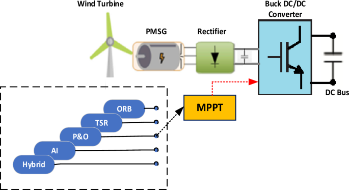
wind variations with a single voltage sensor rather the voltage and current sensors required by the conventional sensored controller. SYSTEM UNDER CONSIDERATION Hereby, the system under

consideration, shown in Fig. 1, is discussed in details14. It is an off-grid WECS that comprises a wind turbine, a gearless Permanent Magnet Synchronous Generator (PMSG), a passive diode

rectifier and a DC/DC converter that bucks the generator rectified voltage to the required DC level and meanwhile acts as the MPP tracker. Table 1 shows considered system parameters. WIND

TURBINE MODEL The mechanical power delivered by a wind turbine (WT), given ideal blades with perpendicular air flow to the rotational plane of the wind turbine, is calculated as

follows14,29; $${P}_{w}=\frac{1}{2}\rho \pi {R}^{2}{C}_{p}(\lambda ,\beta ){{v}_{w}}^{3}$$ (1) where _ρ_ is the air density in kg/m3, _R_ is the turbine blade radius in m, _v__w_ is the wind

velocity striking the turbine blades in m/s and _C__P_ is the turbine power coefficient. It is worth noting that _C__P_ measures the conversion efficiency of the turbine power i.e. the

percentage of power that can be extracted by the WT and is limited by less than 59% as given by Betz limit30. As noted in Eq. (1), _C__P_ depends on _λ_ and _β_ which are the tip speed ratio

and blade pitch angle respectively. λ can be computed from Eq. (2) as follows; $$\lambda = \frac{\omega R}{{v}_{w}}$$ (2) where _ω_ is the wind turbine angular mechanical speed in rad/s.

Figure 2 gives the characteristic curves of harvested mechanical power from the considered WES versus WT speed for different wind speeds. It is clear the that, for each wind speed, there is

an optimal power point at which the WT is forced to operate using a MPPT algorithm to extract the available peak power and maximize system efficiency. After harvesting the maximum mechanical

power, the latter is used to drive a generator to produce the required electrical energy. Due to their high-power density, high efficiency, and direct drive construction, PMSG-based WESs

are an excellent candidate providing a reliable, cost-effective solution16,17. For successful control of generator output power in PMSG-based low-power WESs, a passive rectifier stage

followed by a DC-DC converter stage is found to be a more affordable solution18,19. PMSG MODEL Considering two axis Park’s theory, the state equations governing the PMSG conventional _d_–_q_

model are driven from Fig. 3 as follows31; $$\frac{d{i}_{sd}}{dt}=-\frac{{R}_{sa}}{{L}_{sd}}{i}_{sd}+{\omega }_{s}\frac{{L}_{sq}}{{L}_{sd}}{i}_{sq}-\frac{1}{{L}_{sd}}{v}_{sd}$$ (3)

$$\frac{d{i}_{sq}}{dt}=-\frac{{R}_{sa}}{{L}_{sq}}{i}_{sq}-{\omega }_{s}\frac{{L}_{sd}}{{L}_{sq}}{i}_{sd}{+\omega }_{s}\frac{1}{{L}_{sq}}{\varphi }_{p}-\frac{1}{{L}_{sq}}{v}_{sq}$$ (4) where

\({{i}_{sd, }i}_{sq}\) are the _d-_axis and _q-_axis stator currents respectively, \({R}_{sa}\) is the stator resistance, \({\omega }_{s}\)  is the electrical angular frequency of the

generator;  \({{L}_{sd, }L}_{sq}\) are the stator inductances of generator in the _d_-axis and _q_-axis respectively; \({\varphi }_{p}\) is the permanent flux and  \({{v}_{sd, }v}_{sq}\) are

the _d-_axis and _q-_axis stator voltages respectively. The electromagnetic torque in the rotor (\({T}_{e}\)) is given by; $${T}_{e}=1.5\frac{p}{2}\left[{\varphi

}_{p}{i}_{sq}-{{i}_{sd}i}_{sq}({L}_{sd}-{L}_{sq})\right]$$ (5) where _p_ is the number of poles. PASSIVE RECTIFIER MODEL A full-wave bridge rectifier is applied at the generator output to

convert its output AC voltage into rectified DC voltage \(({V}_{r})\) which is the input voltage \(({V}_{i})\) to the following buck converter stage. The rectified DC voltage is computed

from Eq. (6) as follows32; $${V}_{r}=\frac{3\sqrt{2}}{\pi }{V}_{LL}$$ (6) where \({V}_{LL}\) is the effective value of the rectifier line-to-line input voltage. CONVENTIONAL MPPT CONVERTER

For the considered system, a buck DC/DC converter stage is added after the rectifier stage to step-down the rectifier output DC voltage to the required DC bus level. Meanwhile the switching

of this DC/DC converter stage is controlled to extract the maximum available power at the rectifier output, thus this converter is considered the MPP tracker in the considered system.

Conventionally, a traditional buck converter is applied as the MPPT tracker whose switching is controlled via conventional fixed-step P&O MPPT technique. CONVENTIONAL DC/DC BUCK

CONVERTER MODEL Modeling of conventional buck converter is first carried without employing the input buffer capacitor to verify the buck integrated feature of discontinuous input current.

Then, it is modelled again when applying a buffer capacitor at the buck converter input to emphasize this capacitor importance to buffer enlarged input current ripples and minimize their

propagation to the machine side when using the buck converter as a MPP tracker in RES applications33. For each case, the converter average model is originated, in continuous inductor current

mode, using Fig. 4a and b, to compute voltage and current gains, capacitor ripples voltage ripples \(\Delta {{\varvec{v}}}_{{\varvec{C}}}\), inductor current ripples \(\Delta {i}_{L}\) and

converter input and output current ripples \(\Delta {i}_{i}, \Delta {i}_{o}\) as shown below. It is worth noting that normally in the buck converter model an output capacitor is placed to

filter the obtained output voltage, however, since in the considered application a DC bus or microgrid is considered, thus there is no need for an output capacitor. * To find voltage and

current transfer functions; For both cases; The average inductor voltage _V__L_ = 0, $$\left. \begin{gathered} \therefore \left( {V_{i} - V_{o} } \right)DT - V_{o} \left( {1 - D} \right)T =

0 \hfill \\ \therefore \frac{{V_{o} }}{{V_{i} }} = D \hfill \\ \end{gathered} \right\}$$ (7) Average input power _P__i_ = Average output power _P__o_, $$\left. \begin{gathered} \therefore

V_{i} I_{i} = V_{o} I_{o} \hfill \\ \therefore \frac{{I_{i} }}{{I_{o} }} = \frac{{V_{o} }}{{V_{i} }} = D \hfill \\ \end{gathered} \right\}$$ (8) where _V__i_ and _V__o_ are the converter

input and output voltages respectively, _I__i_ and _I__o_ are the converter input and output currents respectively and _D_ is the converter duty ratio. * To find voltage and current ripples;

For Case I (without _C__i_); When the switch S is closed; $$\left. \begin{gathered} v_{L} = L\frac{{\Delta i_{L} }}{DT} = V_{i} - V_{o} \hfill \\ \therefore \Delta i_{L} = \frac{{V_{o}

\left( {1 - D} \right)T}}{L} = \frac{{V_{o} \left( {1 - D} \right)}}{{f_{sw} L}} \hfill \\ \end{gathered} \right\}$$ (9) $$\Delta {i}_{o}=\Delta

{i}_{L}=\frac{{V}_{o}\left(1-D\right)}{{f}_{sw}L}$$ where _f__sw_ is the converter switching frequency. For Case II (with _C__i_); When the switch S is closed; $$\left. \begin{gathered}

i_{C} = C\frac{{\Delta v_{C} }}{\Delta t} = C\frac{{\Delta v_{C} }}{DT} = I_{i} - I_{o} \hfill \\ \therefore \Delta {\varvec{v}}_{{\varvec{C}}} = \frac{{I_{i} \left( {D - 1}

\right)T}}{{\text{C}}} = \frac{{I_{i} \left( {D - 1} \right)}}{{f_{sw} {\text{C}}}} \hfill \\ \end{gathered} \right\}$$ (10) $$\left. \begin{gathered} v_{L} = L\frac{{\Delta i_{L} }}{DT} =

V_{i} - V_{o} \hfill \\ \therefore \Delta i_{L} = \frac{{V_{o} \left( {1 - D} \right)T}}{L} = \frac{{V_{o} \left( {1 - D} \right)}}{{f_{sw} L}} \hfill \\ \end{gathered} \right\}$$ (11)

$$\Delta {i}_{o}=\Delta {i}_{L}=\frac{{V}_{o}\left(1-D\right)}{{f}_{sw}L}=\frac{{V}_{i}D\left(1-D\right)}{{f}_{sw}L}$$ (12) * Regarding the converter input current, it’s clear that; * In

buck converter without input buffer capacitor _C_i, as shown in Fig. 4a, during the S-OFF mode, no input current exists thus the input current is discontinuous without _C__i__._ * In the

buck converter with input buffer capacitor _C__i_, as shown in Fig. 4b, during S-OFF period, the presence of buffer capacitor forced the converter input current \({i}_{i}\) to be equal to

that capacitor current \({i}_{C}\) in this mode, thus overcoming its discontinuity. However, this capacitor should be relatively large to change the converter input current from

discontinuous to continuous which adds to system cost and losses and affects its reliability. CONVENTIONAL P&O MPPT METHOD Noticeably, P&O MPPT techniques are widely used in WES,

especially for low-cost small-sized standalone ones, for its simplicity and flexibility, in addition to the unnecessity of distributed mechanical speed sensors or anemometers26,26,28, 34.

Its tracking strategy depends on perturbing the generator output rectified voltage or current then observes the change in the extracted power to determine direction of control variable

perturbation. Accordingly, the MPPT converter duty cycle will be continuously perturbed with a predetermined step size, thus regulating the DC voltage or current to maintain operation around

the MPP (zero slope of the power–speed curve)5. Flowchart of the conventional P&O MPPT algorithm is shown in Fig. 5. However, it is worth noting that this method suffers from large

power oscillations around the MPP for large step sizes and sluggish response for small ones35. This problem can be limited using variable step sizes which will be explained later. CONTINUOUS

INPUT/OUTPUT POWER DC/DC BUCK CONVERTERS As previously discussed, the conventional buck converter topology suffers from input current discontinuity which results in high oscillations in the

extracted power, inefficient MPPT and high torque ripples which may affect generator operation. To buffer these oscillations, a large capacitor (_C__i_) is placed at the buck converter

input, yet it affects the entire system life time and reliability as well as increasing its size and cost. To overcome all these limitations, the continuous input/output power DC/DC buck

converters introduced in21 are studied and their average models are derived, in the continuous inductor current mode, to select the one with minimal input current ripples to be adopted in

this study. Voltage and current gains are derived for each converter along with dynamic analysis of each converter to deduce its input and output current ripples as follows; D4 CONVERTER

Modeling of D4 converter, in the continuous inductor current mode, is originated using Fig. 6a. Voltage and current gains are computed then dynamic analysis is carried out to deduce

capacitor voltage ripples \(\Delta {{\varvec{v}}}_{{\varvec{C}}}\), inductors’ ripple currents \(\Delta {i}_{Li}, \Delta {i}_{Lo}\) and input and output current ripples \(\Delta {i}_{i},

\Delta {i}_{o}\) as shown below; * To find voltage and current gains; The average capacitor current _I__c_ = 0, $$\left. \begin{gathered} \therefore \left( {I_{i} - I_{o} } \right)DT + I_{i}

\left( {1 - D} \right)T = 0 \hfill \\ \therefore \frac{{I_{i} }}{{I_{o} }} = D \hfill \\ \end{gathered} \right\}$$ (13) Average input power _P__i_ = Average output power _P__o_, $$\left.

\begin{gathered} \therefore V_{i} I_{i} = V_{o} I_{o} \hfill \\ \therefore \frac{{V_{o} }}{{V_{i} }} = \frac{{I_{i} }}{{I_{o} }} = D \hfill \\ \end{gathered} \right\}$$ (14) * To find the

capacitor voltage ripples and inductors’ ripple currents; When the switch S is closed; $$\left. \begin{gathered} i_{C} = C\frac{{\Delta v_{C} }}{\Delta t} = C\frac{{\Delta v_{C} }}{DT} =

I_{i} - I_{o} \hfill \\ \therefore \Delta {\varvec{v}}_{{\varvec{C}}} = \frac{{I_{i} \left( {D - 1} \right)T}}{{\text{C}}} = \frac{{I_{i} \left( {D - 1} \right)}}{{f_{sw} {\text{C}}}} \hfill

\\ \end{gathered} \right\}$$ (15) $${{v}_{Li}={L}_{i}\frac{\Delta {i}_{Li}}{\Delta t}{=L}_{i}\frac{\Delta {i}_{Li}}{DT}=V}_{i}-{v}_{C}$$ (16) Since, average of inductor voltages = 0

$${\therefore v}_{C}={V}_{i} \pm \Delta {v}_{C}$$ (17) Substitute (17) in (16); $$\left. \begin{gathered} \therefore v_{Li} = L_{i} \frac{{\Delta i_{Li} }}{DT} = \mp \Delta v_{C} \hfill \\

\therefore \Delta i_{Li} = \frac{{\Delta v_{C} DT}}{{L_{i} }} = \frac{{\Delta v_{C} D}}{{f_{sw} L_{i} }} \hfill \\ \end{gathered} \right\}$$ (18) $$\left. \begin{gathered} v_{Lo} = L_{o}

\frac{{\Delta i_{Lo} }}{\Delta t} = L_{o} \frac{{\Delta i_{Lo} }}{DT} = V_{i} - V_{o} \hfill \\ \therefore \Delta i_{Lo} = \frac{{V_{o} \left( {1 - D} \right)T}}{{L_{o} }} = \frac{{V_{o}

\left( {1 - D} \right)}}{{f_{sw} L_{o} }} \hfill \\ \end{gathered} \right\}$$ (19) * To find input and output ripple currents; $$\left. \begin{gathered} \Delta i_{i} = \Delta i_{Li} + \Delta

i_{Lo} = \frac{{ \mp \Delta v_{C} D}}{{f_{sw} L_{i} }} + \frac{{V_{o} \left( {1 - D} \right)}}{{f_{sw} L_{o} }} \hfill \\ \Delta i_{o} = \Delta i_{Lo} = \frac{{V_{o} \left( {1 - D}

\right)}}{{f_{sw} L_{o} }} \hfill \\ \end{gathered} \right\}$$ (20) C1 CONVERTER Modeling of C1 converter, in the continuous inductor current mode, is originated using Fig. 6b. Voltage and

current gains are computed then dynamic analysis is carried out to deduce capacitor voltage ripples \(\Delta {{\varvec{v}}}_{{\varvec{C}}}\), inductors’ ripple currents \(\Delta {i}_{Li},

\Delta {i}_{Lo}\) and input and output current ripples \(\Delta {i}_{i}, \Delta {i}_{o}\) as shown below; * To find voltage and current transfer gains; The average capacitor current _I__c_

=0, $$\left. \begin{gathered} \therefore \left( {I_{i} - I_{o} } \right)DT + I_{i} \left( {1 - D} \right)T = 0 \hfill \\ \therefore \frac{{I_{i} }}{{I_{o} }} = D \hfill \\ \end{gathered}

\right\}$$ (21) Average input power _P__i_ = Average output power _P__o_, $$\left. \begin{gathered} \therefore V_{i} I_{i} = V_{o} I_{o} \hfill \\ \therefore \frac{{V_{o} }}{{V_{i} }} =

\frac{{I_{i} }}{{I_{o} }} = D \hfill \\ \end{gathered} \right\}$$ (22) * To find the capacitor voltage ripples and inductors’ ripple currents; When the switch S is closed; $$\left.

\begin{gathered} i_{C} = C\frac{{\Delta v_{C} }}{\Delta t} = C\frac{{\Delta v_{C} }}{DT} = I_{i} - I_{o} \hfill \\ \therefore \Delta {\varvec{v}}_{{\varvec{C}}} = \frac{{I_{i} \left( {D - 1}

\right)T}}{{\text{C}}} = \frac{{I_{i} \left( {D - 1} \right)}}{{f_{sw} {\text{C}}}} \hfill \\ \end{gathered} \right\}$$ (23) $$\left. \begin{gathered} v_{Li} = L_{i} \frac{{\Delta i_{Li}

}}{\Delta t} = L_{i} \frac{{\Delta i_{Li} }}{DT} = V_{i} - V_{o} \hfill \\ \therefore \Delta i_{Li} = \frac{{V_{i} D\left( {1 - D} \right)T}}{{L_{i} }} = \frac{{V_{i} D\left( {1 - D}

\right)}}{{f_{sw} L_{i} }} \hfill \\ \end{gathered} \right\}$$ (24) $${v}_{Lo}={L}_{o}\frac{\Delta {i}_{Lo}}{\Delta t}{=L}_{o}\frac{\Delta {i}_{Lo}}{DT}={V}_{o}-{v}_{C}$$ (25) Since, average

of inductor voltages = 0 $${\therefore v}_{C}={V}_{i} \pm \Delta {v}_{C}$$ (26) Substitute (26) in (25); $$\left. \begin{gathered} \therefore v_{Lo} = L_{o} \frac{{\Delta i_{Lo} }}{DT} =

V_{o} - V_{i} \mp \Delta v_{C} \mathop \Rightarrow \limits^{{\Delta v_{C} \downarrow \downarrow }} L_{o} \frac{{\Delta i_{Lo} }}{DT} = V_{o} - V_{i} \hfill \\ \therefore \Delta i_{Lo} =

\frac{{V_{o} \left( {D - 1} \right)T}}{{L_{o} }} = \frac{{ - V_{o} \left( {1 - D} \right)}}{{f_{sw} L_{o} }} \hfill \\ \end{gathered} \right\}$$ (27) * To find input and output ripple

currents; $$\left. \begin{gathered} \Delta i_{i} = \Delta i_{Li} = \frac{{V_{i} D\left( {1 - D} \right)}}{{f_{sw} L_{i} }} \hfill \\ \Delta i_{o} = \Delta i_{Li} - \Delta i_{Lo} =

\frac{{V_{i} D\left( {1 - D} \right)}}{{f_{sw} L_{i} }} + \frac{{V_{o} \left( {1 - D} \right)}}{{f_{sw} L_{o} }} \hfill \\ \end{gathered} \right\}$$ (28) D6 CONVERTER Modeling of D6

converter, in the continuous inductor current mode, is originated using Fig. 6c. Voltage and current gains are computed then dynamic analysis is carried out to deduce capacitor voltage

ripples \(\Delta {{\varvec{v}}}_{{\varvec{C}}}\), inductors’ ripple currents \(\Delta {i}_{Li}, \Delta {i}_{Lo}\) and input and output current ripples \(\Delta {i}_{i}, \Delta {i}_{o}\) as

shown below; * To find voltage and current transfer functions; The average capacitor current _I__c_ = 0, $$\left. \begin{gathered} \therefore \left( {I_{i} - I_{o} } \right)DT + I_{i} \left(

{1 - D} \right)T = 0 \hfill \\ \therefore \frac{{I_{i} }}{{I_{o} }} = D \hfill \\ \end{gathered} \right\}$$ (29) Average input power _P__i_ = Average output power _P__o_, $$\left.

\begin{gathered} \therefore V_{i} I_{i} = V_{o} I_{o} \hfill \\ \therefore \frac{{V_{o} }}{{V_{i} }} = \frac{{I_{i} }}{{I_{o} }} = D \hfill \\ \end{gathered} \right\}$$ (30) * To find the

capacitor voltage ripples and inductors’ ripple currents; When the switch S is closed; $$\left. \begin{gathered} i_{C} = C\frac{{\Delta v_{C} }}{\Delta t} = C\frac{{\Delta v_{C} }}{DT} =

I_{i} - I_{o} \hfill \\ \therefore \Delta {\varvec{v}}_{{\varvec{C}}} = \frac{{I_{i} \left( {D - 1} \right)T}}{{\text{C}}} = \frac{{I_{i} \left( {D - 1} \right)}}{{f_{sw} {\text{C}}}} \hfill

\\ \end{gathered} \right\}$$ (31) $${{v}_{Li}={L}_{i}\frac{\Delta {i}_{Li}}{\Delta t}{=L}_{i}\frac{\Delta {i}_{Li}}{DT}=V}_{i}-{v}_{C}$$ (32) Since, average of inductor voltages = 0

$${\therefore v}_{C}={V}_{i} \pm \Delta {v}_{C}$$ (33) Substitute (33) in (32) $$\left. \begin{gathered} \therefore v_{Li} = L_{i} \frac{{\Delta i_{Li} }}{DT} = \mp \Delta v_{C} \hfill \\

\therefore \Delta i_{Li} = \frac{{{ }\Delta v_{C} DT}}{{L_{i} }} = \frac{{\Delta v_{C} D}}{{f_{sw} L_{i} }} \hfill \\ \end{gathered} \right\}$$ (34) $${v}_{Lo}={L}_{o}\frac{\Delta

{i}_{Lo}}{\Delta t}{=L}_{o}\frac{\Delta {i}_{Lo}}{DT}={v}_{C}-{V}_{o}$$ (35) Substitute (33) in (35); $$\left. \begin{gathered} v_{Lo} = L_{o} \frac{{\Delta i_{Lo} }}{DT} = V_{i} \pm \Delta

v_{C} - V_{o} \mathop \Rightarrow \limits^{{\Delta v_{C} \downarrow \downarrow }} v_{Lo} \cong V_{i} - V_{o} \hfill \\ \therefore \Delta i_{Lo} = \frac{{V_{o} \left( {1 - D}

\right)T}}{{L_{o} }} = \frac{{V_{o} \left( {1 - D} \right)}}{{f_{sw} L_{o} }} \hfill \\ \end{gathered} \right\}$$ (36) * To find input and output ripple currents; $$\left. \begin{gathered}

\Delta i_{i} = \Delta i_{Li} = \frac{{\Delta v_{C} D}}{{f_{sw} L_{i} }} \hfill \\ \Delta i_{o} = \Delta i_{Lo} = \frac{{V_{o} \left( {1 - D} \right)}}{{f_{sw} L_{o} }} \hfill \\

\end{gathered} \right\}$$ (37) Table 2 summarizes the considered buck converters' performance parameters. It’s vivid that the D4, C1 and D6 converters feature continuous input current

unlike the conventional buck converter, thus eliminating the required buffer capacitor at converter input which in turn increases system lifetime and reduces its size and cost. However,

these three converters differ regarding the input current ripples which are mirrored in the extracted power oscillations thus affecting the extracted power value and the converter tracking

performance. Referring to Table 2, D6 converter experiences the least input current ripples i.e. the least tracked power oscillations. Thus, it will be selected to be applied in the

considered WECS, instead of the conventional buck converter, to eliminate the need of buffer capacitor and meanwhile minimize power oscillations and maximize the tracked power. Comparing

buck converter with input buffer capacitor to D6 converter, the latter shows superior performance. This can be concluded from converters’ modes of operation shown in Figs. 4b and 6c

respectively and derived ripples’ equations presented in Table 2. Regarding capacitor voltage ripples, in both cases, it depends on converter input current as deduced from Table 2. However,

although a relatively large buffer capacitor is placed at buck converter input to overcome its discontinuity, still high ripples in input current exist resulting in large input voltage

ripples and in turn large capacitor voltage ripples since the buffer capacitor is placed directly in parallel to converter input. Oppositely, in D6, the capacitor is separated from converter

input by an input inductor which filters input current resulting in minimal capacitor voltage ripples. Hence a comparatively quite smaller linkage capacitor is required in D6 than that

required at the buck converter input. Regarding inductor current ripples, it’s clear from Table 2 that D6 input inductor current ripples, \(\Delta {i}_{Li}= \frac{{\Delta

v}_{C}D}{{f}_{sw}{L}_{i}}\), which is meanwhile the converter input current, just depends on the small capacitor voltage ripples, unlike the buck inductor current ripples which depend on

converter input rippled voltage, \({\Delta i}_{L}=\frac{{V}_{i}D(1-D)}{{f}_{sw}L}\). Moreover, an additional output inductor exists in D6 to aid the input one resulting in low sizes for

input and output inductor of D6, compared to that of buck inductor. PROPOSED MPPT CONVERTER As previously discussed, D6 CICO power converter is applied in the considered WECS as it features

minimal input current ripples. Thus, maximum tracking efficiency can be achieved without the need of buffer capacitor which reduces system size and cost and enhances system reliability. To

add to these merits, D6 converter acting as the MPP tracker will use a variable-step P&O scheme to solve the tradeoff between tracking speed and accuracy. Finally, another modification

is proposed to D6 control in order to eliminate the need for a current sensor by estimating the DC rectified current from D6 derived averaged state space model rather than directly measuring

it. Hence, current sensorless MPPT is achieved to add to system cost effectiveness and compact size. D6 AVERAGED STATE SPACE MODEL The State Space Averaging method is widely used by the

power electronics industry giving quite insight into the converter behavior36. The dynamic small signal model of D6 is derived based on its averaged state-space model which is divided into

two sub-models, each addressing certain converter dynamics. The first sub-model analyzes the converter behavior when the converter switch (S) is at the ON state (i.e. switching period from

0: DT) while the second sub-model offers converter dynamics when the switch (S) is at OFF (i.e. switching period from DT: T). For each region, the corresponding state-space sub-model is

deduced and finally the total state-space model, averaged along the total switching period, is derived. Inductors and capacitor’s internal resistances are neglected for sake of simplicity. *

_State-space sub-model when Switch “S” is ON_ From Fig. 6c, during switching ON period (t = 0-DT), the following state-space equations can be derived;

$${i}_{C}=C\frac{d{v}_{c}}{dt}={i}_{Li}-{i}_{Lo}$$ (38) $${v}_{Lo}={L}_{o}\frac{d{i}_{Lo}}{dt}={v}_{C}-{V}_{DC-bus}$$ (39) $${v}_{Li}={L}_{i}\frac{d{i}_{Li}}{dt}= {V}_{r} -{v}_{C}$$ (40)

$${y= {I}_{r}=i}_{Li}$$ (41) where \({V}_{DC-bus}\) is the DC bus voltage at D6 converter output (\({V}_{DC-bus}={V}_{o}\)) and it is constant = 400 V while \({V}_{r}\) is the generator

rectified voltage which is input to D6 converter (\({V}_{r}={V}_{i}\)) and has to be regulated by the MPPT controller to force operation around the MPP. Both \({V}_{DC-bus}\) and \({V}_{r}\)

are considered model inputs. _y_ is the model output which is the generator rectified current \({I}_{r}\) which is meanwhile D6 input current _I__i_. This current is to be estimated by the

sensorless MPPT controller rather than being sensed thus eliminating its sensor. Equations (38–41) are rearranged to obtain the linear time-invariant state-space sub-model given by; $$\left.

\begin{gathered} \left[ {\begin{array}{*{20}c} {\dot{v}_{c} } \\ {i_{{{L}o}} } \\ {i_{{{L}i}} } \\ \end{array} } \right] = A_{1} \left[ {\begin{array}{*{20}c} {v_{C} } \\ {i_{Lo} } \\

{i_{Li} } \\ \end{array} } \right] + B_{1} \left[ {\begin{array}{*{20}c} {V_{DC - bus} } \\ {V_{r} } \\ \end{array} } \right] \hfill \\ y = C_{1} \left[ {\begin{array}{*{20}c} {v_{C} } \\

{i_{Lo} } \\ {i_{Li} } \\ \end{array} } \right] \hfill \\ \end{gathered} \right\}$$ (42) where $${A}_{1}=\left[\begin{array}{ccc}0& -\frac{1}{C}& \frac{1}{C}\\ \frac{1}{{L}_{o}}&

0& 0\\ -\frac{1}{{L}_{i}}& 0& 0\end{array}\right], {B}_{1}=\left[\begin{array}{cc}0& 0\\ -\frac{1}{{L}_{o}}& 0\\ 0&

\frac{1}{{L}_{i}}\end{array}\right],\;and\;{C}_{1}=\left[\begin{array}{ccc}0& 0& 1\end{array}\right]$$ * _State-space sub-model when Switch “S” is OFF_ From Fig. 6c, during switching

OFF period (t = DT-T), the following state-space equations can be derived; $${i}_{C}=C\frac{d{v}_{c}}{dt}={i}_{Li}$$ (43) $${v}_{Lo}={L}_{o}\frac{d{i}_{Lo}}{dt}=-{V}_{DC-bus}$$ (44)

$${v}_{Li}={L}_{i}\frac{d{i}_{Li}}{dt}= {V}_{r}-{v}_{C}$$ (45) $${y= {I}_{r}= i}_{Li}$$ (46) Equations (43–46) are rearranged to obtain the linear time-invariant state-space sub-model given

by; $$\left. \begin{gathered} \left[ {\begin{array}{*{20}c} {\dot{v}_{c} } \\ {i_{{{L}o}} } \\ {i_{{{L}i}} } \\ \end{array} } \right] = A_{2} \left[ {\begin{array}{*{20}c} {v_{C} } \\

{i_{Lo} } \\ {i_{Li} } \\ \end{array} } \right] + B_{2} \left[ {\begin{array}{*{20}c} {V_{DC - bus} } \\ {V_{r} } \\ \end{array} } \right] \hfill \\ y = C_{2} \left[ {\begin{array}{*{20}c}

{v_{C} } \\ {i_{Lo} } \\ {i_{Li} } \\ \end{array} } \right] \hfill \\ \end{gathered} \right\}$$ (47) where $${A}_{2}=\left[\begin{array}{ccc}0& 0& \frac{1}{C}\\ 0& 0& 0\\

-\frac{1}{{L}_{i}}& 0& 0\end{array}\right], {B}_{2}=\left[\begin{array}{cc}0& 0\\ -\frac{1}{{L}_{o}}& 0\\ 0&

\frac{1}{{L}_{i}}\end{array}\right],\;and\;{C}_{2}=\left[\begin{array}{ccc}0& 0& 1\end{array}\right]$$ * _Averaged state-space model_ For a clear insight of entire system dynamics,

the total system averaged state-space model is found to be; $$\left. \begin{gathered} \dot{x} = \overline{A}x + \overline{B}u \hfill \\ y = \overline{C}x \hfill \\ \end{gathered} \right\}$$

(48) where $$\left. {\begin{array}{*{20}c} {\overline{A} = A_{1} *d + A_{2} *\left( {1 - d} \right)} \\ {\overline{B} = B_{1} *d + B_{2} *\left( {1 - d} \right)} \\ {\overline{C} = C_{1} *d

+ C_{2} *\left( {1 - d} \right)} \\ \end{array} } \right\}$$ and _D_ is the instantaneous value of D6 converter duty ratio. Hence, applying the latter to system state space sub-models,

presented in (42) and (47), the total averaged state-space model of the proposed system is given by (49); $$\left. \begin{gathered} \left[ {\begin{array}{*{20}c} {\dot{v}_{c} } \\

{i_{{{L}o}} } \\ {i_{{{L}i}} } \\ \end{array} } \right] = \overline{A}\left[ {\begin{array}{*{20}c} {v_{C} } \\ {i_{Lo} } \\ {i_{Li} } \\ \end{array} } \right] + \overline{B}\left[

{\begin{array}{*{20}c} {V_{DC - bus.} } \\ {V_{r} } \\ \end{array} } \right] \hfill \\ y = \overline{C}\left[ {\begin{array}{*{20}c} {v_{C} } \\ {i_{Lo} } \\ {i_{Li} } \\ \end{array} }

\right] \hfill \\ \end{gathered} \right\}$$ (49) where $$\overline{A }=\left[\begin{array}{ccc}0& -\frac{1}{C}d& \frac{1}{C}\\ \frac{1}{{L}_{o}}d& 0& 0\\

-\frac{1}{{L}_{i}}& 0& 0\end{array}\right], \overline{B }=\left[\begin{array}{cc}0& 0\\ -\frac{1}{{L}_{o}}& 0\\ 0& \frac{1}{{L}_{i}}\end{array}\right],\;and\; \overline{C

}=\left[\begin{array}{ccc}0& 0& 1\end{array}\right]$$ Based on the derived averaged state-space model of the selected D6 converter, the state space block diagram, shown in Fig. 7,

is obtained. This diagram is the base upon which the proposed sensorless MPPT scheme is realized since the output of this model is the rectified input current of D6 converter which will be

estimated using this model rather than being directly sensed using a current sensor. Conclusively, the derived averaged state-space model of D6 is used to estimate the converter input

current which will be injected into the sensorless MPPT process to track the maximum power of the considered WECS. This will save the cost of the eliminated current sensor which enhances

system cost-effectiveness. PROPOSED SENSORLESS MPPT A current sensorless MPPT scheme is proposed which consists of two main stages. In the first stage, the rectified DC current is estimated

from D6 averaged state-space model derived in the previous subsection, rather than directly measuring it through a DC current sensor. Then in the second stage, the estimated rectified

current along with the measured rectified voltage are utilized by a variable step P&O MPPT algorithm to extract the maximum available power and force converter operation around the MPP.

The two stages are discussed in details as follows. * 1. Current estimation stage The first stage is responsible for observing and estimating the rectified generator current which is the

converter input current from D6 averaged state-space-based dynamic model which is derived in the previous section. However, to achieve this, the derived model should be checked for its

observability i.e. to ensure system capability of using model input and output to estimate the converter rectified current from the derived model to be injected later in the MPPT process.

For the system to be completely state observable, the observability matrix Qo of dimension _n*n_ has to be full column rank i.e. its rank = _n_37. This means that the matrix has _n_

independent pivot columns which occurs when it has a non-zero determinate i.e. \(\left|{{\varvec{Q}}}_{{\varvec{o}}}\right|\ne 0\) as shown below37; $$Observability\;matrix,{ }Q_{o} = \left[

{\begin{array}{*{20}c} C \\ {CA} \\ {CA^{2} } \\ : \\ : \\ {CA^{n - 1} } \\ \end{array} } \right]\mathop \Rightarrow \limits^{{\left| {{\varvec{Q}}_{{\varvec{o}}} } \right| \ne 0}}

System\;is\;completely\;state\;observable$$ So, to check the observability of D6 derived model, first the observability matrix _Q__o_ is computed as follows; $$\left. \begin{gathered} CA =

\left[ {\begin{array}{*{20}c} { - \frac{1}{{L_{i} }}} & 0 & 0 \\ \end{array} } \right] \hfill \\ CA^{2} = CAA = \left[ {\begin{array}{*{20}c} 0 & {\frac{1}{{L_{i} C}}d} & { -

\frac{1}{{L_{i} C}}} \\ \end{array} } \right] \hfill \\ \therefore Q_{o} = \left[ {\begin{array}{*{20}c} 0 & 0 & 1 \\ { - \frac{1}{{L_{i} }}} & 0 & 0 \\ 0 &

{\frac{1}{{L_{i} C}}d} & { - \frac{1}{{L_{i} C}}} \\ \end{array} } \right] \hfill \\ \end{gathered} \right\}$$ (50) Hence, for an observable model from which the converter input current

can be estimated \(\left|{{\varvec{Q}}}_{{\varvec{o}}}\right|\ne 0 \to -\frac{d}{{L}_{i}^{2}C}\ne 0\) i.e. the duty ratio _d_ \(\ne 0\). Thus, the converter input current can be estimated

rather than being directly sensed, eliminating the current senor. To realize the current online estimation, the small signal model, shown in (49), is represented by the block diagram shown

in Fig. 7. This block diagram presents the model in a block form rather than in matrix form thus simplifying the sensorless scheme realization. As concluded from the block diagram, the model

output _I__r_, which is the estimated rectified current input to D6, is estimated by measuring solely the rectified voltage _V__r_ given that DC-bus voltage is constant. Thus, the current

sensor can be eliminated and this control block can be implemented on a simple controller to substitute for the current sensor absence. The predicted current signal along with the measured

voltage signal are fed to the controller second stage which is responsible for MPPT as described later. Figure 8 shows the conventional sensored MPPT controller versus the proposed

sensorless variable step one. Unlike the conventional single-stage MPP controller which requires both voltage and current sensors, the proposed sensorless controller requires only one

voltage sensor and includes two sequential stages; current estimation stage followed by MPPT stage. Thus, the proposed current sensorless MPPT scheme has the capabilities of eliminating the

current senor thus reducing the MPP controller cost and size as well as achieving noise immunity. * 2. MPPT stage The second following stage employs variable-step P&O-based MPPT

algorithm to maintain the operation around the MPP. As previously discussed in the P&O scheme, the rectifier output power versus the rectified voltage is amended to operate at the zero

slope for the _P–V_ curve. However, for fixed step sizes38,39, larger step sizes result in oscillation near the MPP affecting tracking accuracy while smaller step sizes increase the tracking

time and slow down the response. Thus, to solve the tradeoff between tracking accuracy and convergence speed, much research was introduced to apply steps with varying sizes according to

region of operation7. Some use variable step sizes40,40,41,43, others use adaptive44,45 or hybrid ones46. The variable step size shown in Eq. (51) is a well-known solution to the conflict

between tracking accuracy and convergence speed in PV/wind systems where both have a _P_–_V_ curve that has an optimal MPP at certain environmental condition7,22. Meanwhile, it features

easier realization than adaptive and hybrid step sizes which require more tuning and design7. This variable step depends on the slope of the tracked _P_–_V_ curve (i.e. tracked power change

divided by the tracked voltage change) which is big away from the MPP then gets smaller towards that optimal point (at which the slope of the curve = 0)22. Thus, larger-speed step sizes are

applied in regions away from the MPP while small step sizes are utilized near the MPP as shown in Fig. 9. This eliminates the drawbacks of fixed step sizes (slow tracking for small fixed

step sizes and large power oscillations around the MPP for large fixed step sizes) and enhances the WECS MPPT performance, maximizing the captured power, improving the settling time and

reducing the oscillation level. Thus, for direct converter control, the conventionally adopted variable step-size \(\Delta D\) is shown in (51); $$\Delta D={N}_{1}\left|\frac{\Delta

P}{\Delta V}\right|$$ (51) where $$\Delta P=P\left(k\right)-P(k-1)$$ $$\Delta V=V\left(k\right)-V(k-1)$$ $$\Delta D=D\left(k\right)-D(k-1)$$ and _N_1 is the scaling factor designed only once

at the start of operation. The same concept is employed but depending on the slope of the tracked _P-I_ curve in WES (_dP_/_dI_)40 while in42 it depends on the slope of mechanical power of

the WT versus speed (_dP_/_dω_). However, the conventional variable step-size, being dependent on the division of PV power change by PV voltage change _(∆P_/_∆V_), can affect the MPPT

performance due to this step size digression, particularly under sudden power changes due to the division issue36. Thus, in this paper, the variable step size is modified to depend solely on

\(\left|\Delta {\text{P}}\right|\) rather than \(\left|\frac{\Delta {\text{P}}}{\Delta V}\right|\) as shown in (52); $$\Delta D={N}_{2} \left|\Delta {\text{P}}\right|$$ (52) This will

eliminate division computations burden and also enhance the tracking performance as illustrated in Fig. 10. For a change occurring in wind speed, the operating point shifts from ‘X’ to ‘Y’.

Thus, a change in rectified current (_∆I_) occurs reducing the tracked power while almost no _∆V_ takes place. For a successful transfer to the new MPP ‘M’, the considered MPPT algorithm

must decrement the duty ratio _D_ by a convenient step size. * For the widely used _∆P_/_∆V_ step, an almost zero _∆V_ occurs which in turn causes a vast increase in the adopted step-size.

Hence, the duty ratio _D_ noticeably decrements shifting operation to ‘Z’ which consequently results in longer tracking time till reaching ‘M’ and a considerable transient power loss. * For

the proposed _∆P_ step, division by _∆V_ is avoided, thus overcoming the large increase in the step-size. Thus, the operating point is shifted to ‘N’ which is close to the MPP ‘M’, reducing

transient power loss and speeding up the tracking process. Conclusively, the employed variable step-size minimizes tracked power ripples, enhances MPPT dynamics and simplifies control

complexity due to the eliminated division computation. Thus, the proposed sensorless MPPT controller, adopting variable-step P&O algorithm, can give satisfactory performance yet with

minimum complexity for easier implementation on low-cost microcontrollers. The adopted variable step-size, given by Eq. (52), besides solving the trade-off issue, it depends solely on

tracked power change _∆P_ rather than the ratio _∆P_/_∆V_, thus eliminating division computations and high-power fluctuations around the MPP. Adding to all of this, elimination of current

sensor adds to system compactness and cost-effectiveness. SIMULATION RESULTS To verify the ability of selected D6 converter to minimize input current and power ripples at reduced component

sizes and least conversion losses, the considered off-grid WES is simulated using MATLAB/Simulink once using the conventional buck converter (with buffer input capacitor of 220 µF and

inductor of 10 mH), then again using D6 converter with reduced size passive elements (_L_1 = _L_2 = 1 mH and _C_ = 10 uF). This is realized under two step changes in wind speed from 12 to 10

m/s at t = 1 s, then from 10 to 11 m/s at _t_ = 2 s in order to confirm the effectiveness of the employed sensored variable-step P&O MPPT technique during sudden changes. Figure 11

shows system simulation results using the basic buck converter while Fig. 12 demonstrates those of D6 converter. Simulation results include generator torque and mechanical power, converter

input current, converter average input tracked power and converter average output power. Table 3 summarizes simulation results’ parameters that include the attained torque ripples \(\Delta

{\varvec{T}}\), mechanical power ripples \(\Delta {P}_{mech}\), converter input current ripples \(\Delta {I}_{i}\), converter average input power and its ripples \({P}_{i},\Delta {P}_{i}\)

and converter average output power and its ripples \({P}_{o},\Delta {P}_{o}\) for each of the two converters. The converter average input power \({P}_{i}\) shows the power that was

successfully tracked by the converter and available at its input where its value is enhanced by the converter ability to minimize the input current ripples. Finally, the converter efficiency

which is affected by the converter switching and copper losses is computed by (53). The less the inductor size, the less their copper losses, thus the more available power at the converter

output \({P}_{o}\). $${\mathrm{\%}\xi }_{conversion}=\frac{{P}_{o}}{{P}_{i}}\left(100\right)$$ (53) Analyzing Figs. 11 and 12 parts along with Table 3 parameters, both converters were able

to adequately track the MPP, during different wind speeds, which validates the applied sensored variable-step P&O scheme. However, there were differences in performance between both

converters as explained below. First regarding the inductor and capacitor sizes, the ones included in the basic buck converter have relatively larger values than those in D6, thus more cost,

size and losses. This was selected to reduce the effect of the input current discontinuity of the basic buck converter on its MPPT performance, yet at the cost of more losses and reduced

lifetime. Moreover, the basic converter shows relatively slower tracking time than that of D6 due to its larger passive elements which increase the time constant and in turn slows down the

response as concluded from Table 3 regarding the less settling time attained by D6 during both step changes. Despite its larger size passive elements, still noticeably large fluctuations in

the buck converter input current exist as shown in Fig. 11c compared to those of D6 input current given by Fig. 12c. These ripples are reflected in the relatively large fluctuations in the

generator torque and mechanical power of the basic buck converter (Fig. 11a and b respectively) when compared to those of D6 (Fig. 12a and b respectively), as presented in Table 3, which in

turn affects turbine safety. On the other hand, the less fluctuations in D6 converter reduces stresses on the machine and maintains its lifetime. Moreover, the larger input current ripples

in basic buck converter are also mirrored in considerably more power ripples at the converter input thus reducing the available tracked input power (Fig. 11d) when compared to the available

input power of D6 with its minimal oscillations (Fig. 12d). This enhanced the tracking performance of D6 during different wind speeds. Finally, the relatively less size passive elements

included in D6 feature less losses i.e. more power available at the converter output during different wind speeds (Fig. 12e when compared to that of basic buck (Fig. 11e). Thus, as shown in

Table 3, D6 exceled in the conversion efficiency achieved, experiencing ≥ 99% at different wind speeds. Moreover, remarkable increase in D6 output power can be noticed when compared to that

of the traditional buck converter i.e. D6 output power exceeds that of basic buck converter by almost 550, 340, and 60 W at wind speed of 12, 11 and 10 m/s respectively. These enhancements

are related to D6 converter outstanding property of continuous input current which is further reflected on minimal ripples in the converter input power and more available power to be tracked

in addition to eliminating the need of the buffer large capacitor. Thus, the whole system reliability, efficiency and tracking time are enhanced along with reducing stresses on machine.

Another experiment is carried out to verify the effectiveness of the proposed sensorless variable-step P&O MPPT scheme. In this experiment, the superior D6 converter is again tested

using MATLAB/Simulink under the two considered step changes of wind speed but when applying the proposed sensorless MPPT scheme based on its derived state space averaged model of D6

converter. Figure 13a–e shows D6 simulation results, when applying the proposed sensorless MPPT scheme, regarding generator torque and mechanical power, converter input current, converter

average input tracked power and converter average output power respectively while the third column of Table 3 summarizes D6 performance parameters for these simulation results. It can be

concluded that using the proposed sensolress MPPT scheme, D6 successfully tracked the MPP during different wind speeds which validates the proposed scheme principle. However, longer tracking

time and more ripples are noticed with D6 when using the sensorless controller rather than the sensored one. This can be related to the computations burden and time required to estimate the

converter input current value by the sensorless scheme. Despite the small differences between both controllers’ response, the overall performance of both is quite close verifying the

proposed sensorless one effectiveness due to its less cost and size. Moreover, D6 converter applying the sensorless scheme still outweighs the basic converter regarding the tracking time,

the ripples attained in the applied torque, mechanical power and input current as well as the input and output converter powers’ values. It was able to achieve conversion efficiencies of

more than 99% during different wind speeds. In summary, simulation results demonstrated how the selected CICO D6 converter outweighs the conventional buck one regarding current continuity,

minimal electrical and mechanical power ripples and enhanced system reliability and efficiency yet at considerably less capacitor and inductor values. Moreover, the effectiveness of proposed

sensorless controller is verified in tracking the MPP during different wind speeds with quite acceptable performance parameters adding to system compactness and cost effectiveness due to

the eliminated current sensor. DISCUSSION Generally, small sized decentralized wind energy-based power generation systems require efficient and reliable MPP tracker realized with simple

implementation and low-cost microcontrollers. Thus, in this paper, the considered standalone PMSG-based WECS adopts a continuous input current buck converter featuring minimal input current

ripples without the need input buffer capacitor, thus system reliability and tracking efficiency are enhanced. Moreover, a current sensorless MPPT controller, based on variable step P&O

algorithm, is proposed to add to system simplicity and reduced cost as well as compromise between the tracking time and accuracy. The proposed system capabilities can be summarized as

follows; * Selected D6 converter Among continuous input current buck converters, D6 converter was selected since it features the least input current ripples, as verified from the derived

average models of these converters. This results in least fluctuations in the tracked power and better tracking performance. Compared to traditional two-passive elements buck converter, the

selected three-element D6 converter, despite its greater component-count, features less cost, losses and enhanced reliability as well as better MPPT performance as demonstrated below.

According to Table 4, the values of passive elements selected in simulation work for the buck converter and D6 are listed. It’s clear that the input capacitor and output inductor of the

conventional buck converter outsize those of D6 converter (the converter capacitor and input and output inductors). Despite these relatively larger values, more input current and power

ripples have resulted in case of the basic buck converter as verified by simulation results. However, if larger values for buck converter elements are to be selected, system cost and size

will greatly increase and the system will be cost-ineffective. Thus, values shown in Table 4 are adopted. Although there may be some variations in selected elements’ sizes in real-time

implementation, yet still buck converter will possess elements of larger size than those of D6. So, the objective of this comparison is to show the effect of element size on element cost and

losses and that although D6 is a three-passive element converter, it is less in cost and losses than the two-element buck since it acquires less elements size. For fair comparison, same

operating conditions are considered as well as same components’ manufacturer in both converters w.r.t to each element type (capacitor or inductor). * i. _Cost_ Regarding the cost issue, it

varies according to different aspects, mainly component size and operating voltage/current level. According to values presented it Table 4, the cost of each converter passive component is

decided based on the prices shown on the website of the trust-worthy electric components’ store; “Mouser electronic components”, Available at: https://eu.mouser.com/. * Capacitors’ cost The

input capacitor of the buck converter should withstand operating voltage of almost 620 V which is the rectified voltage _V__r_, at the converter input (_P__r_/_I__r_ = 15500 W/25 = 620 V).

Thus, a 220 µF, 620 V capacitor is required. For cost-effectiveness, an electrolytic capacitor with close specifications (220 uF, 630 V) was found for almost 8€ as shown in Table 5. So, it

was selected, yet at the limitation of more size and weight as well as less lifetime and reliability than a corresponding film one due to high input current ripples at the converter input

where it is placed. For better reliability, the electrolytic capacitor can be replaced by a film capacitor featuring close specifications of 225 uF, 700 V yet at a higher cost of 85.74€

which is more than ten times that of the electrolytic one as shown in Table 5. Regarding D6 converter with same operating conditions only 10 µF is required as per Table 4. Thus, a film

capacitor of close specifications (220 µF, 630 V) is chosen for its reliability and relatively much less cost of 4,15€ which is half the cost of buck electrolytic converter and twenty times

less than buck film capacitor cost as shown in Table 5. This is related to the smaller size of D6 capacitor compared to that of buck. * Inductors’ cost The conventional buck output inductor

should withstand operating current of almost 40 A which is the converter output current (_P_/Vo = 15500 W/400 = 39 A). Thus, according to Table 4 values, a 10 mH, 40 A inductor is required

for buck converter whereas for D6, a 1 mH, 40 A output inductor and 1 mH, 25 A input inductor are required. However, according to components availability, the following was found at Mouser

website; For buck converter, a 50 A, 10 mH, 0.023 Ω power inductor is available for 760€ whereas for D6 input inductor, a 30 A, 1 mH, 0.009 Ω is available for 96€ and a 50 A, 1 mH, 0.005 Ω

for 163.6€ is available for D6 output inductor as shown in Table 6. Hence, it’s clear that the cost of D6 both inductors’ (260€) is still almost three times less than the cost of the single

buck inductor due to its larger size. Moreover, the 10mH buck inductor features resistance of 0.023 Ω which is almost five times that of D6 output inductor and 3.5 times that of D6 input

inductor as concluded from Table 6 which results in more losses in buck converter. To reduce the inductor cost, a 50 A, 1 mH, 0.0017 Ω common mode choke inductor is available at 11.45€, yet

at the size of 1mH and not available in bigger sizes. Hence, it can be used for the input and output inductors of D6 with total cost of 2*11.45€. However, when applied with the buck, it can

be used as a series patch of 10 inductor units to realize total of 50 A, 10*1 mH, 10*0.0017 Ω inductor yet at a bigger size and weight as well as five times the cost of that of D6 in

addition to more resistive losses. Conclusively, the larger capacitor and inductor sizes featured by the two-element buck converter cost way more than those of the three-element D6 due to

the latter relatively much smaller sizes. * ii. _Losses_ As per resistive power losses associated with converters’ capacitors, almost close ESR resistances are experienced in the film

capacitor associated with buck or D6, yet the high voltage ripples buffered by buck capacitor can increase its losses. However, for cost-effectiveness, if an electrolytic capacitor is used

with buck, it features a quite bigger ESR resistance as shown in Table 5 i.e. more losses. Normally, electrolytic capacitors have larger internal power loss for same amount of ripple current

compared to film ones47. Regarding resistive power losses experienced by converters’ power inductors, the input and output power inductors of D6 exert relatively less resistances values

(_R__Li_ = 0.009 Ω, _R__Lo_ = 0.005 Ω) compared to that of buck output inductor (_R__L_ = 0.023 Ω), as shown in Table 6, resulting in total average power losses for both D6 inductors

altogether less than that exerted by the buck single inductor. For _I__i_ = 25 A and _I__o_ = 40 A, $$For\;D6;P_{loss - D6} = I_{i}^{2} \left( {0.009} \right) + I_{o}^{2} \left( {0.005}

\right) = 13.6\;{\text{W}}\;whereas\;for\;buck\;P_{loss - buck} = I_{o}^{2} \left( {0.023} \right) = 36.8\;{\text{W}}$$ As per losses experienced by converters’’ choke inductors, the average

losses exerted by buck converter inductor units are quite larger than those of D6 input and output inductors altogether since buck is made of 10 series inductor units as shown in Table 6

while each inductor in D6 is a single unit (as in simulation case). For _I__i_ = 25 A and _I__o_ = 40 A, \(For\;D6;P_{loss - D6} = I_{i}^{2} \left( {0.0017} \right) + I_{o}^{2} \left(

{0.0017} \right) = 3.78\;{\text{W}}\;whereas\;for\;buck\;P_{loss - buck} = 10I_{o}^{2} \left( {0.0017} \right) = 27.2\;{\text{W}}\) Conclusively, although buck has two passive elements

rather than the three-element D6, it acquires more resistive power losses due to its components’ relatively larger size. * iii. _Reliability_ As previously explained in the cost aspect, for

cost effectiveness, the buck film capacitor can be replaced by electrolytic capacitor. However, electrolytic capacitors experience less lifetime affecting reliability in case of high current

ripples which is the case of the buck converter47. The application of excessive mechanical stress or excessive electrical parameters such as operating voltage and ripple currents cause poor

contact or open circuits in electrolytic capacitors causing its degradation & shortens its life span48. * iv. _MPPT performance_ Although the buck converter features larger passive

elements than those of D6, still it experiences larger input current ripples as shown in Fig. 11c compared to that of D6, Fig. 12c due to buck converter inherited feature of pulsating input

current. This results in larger ripples in the power tracked by buck converter, more losses and less captured power which affects system efficiency as concluded from simulation results

summarized in Table 3. Moreover, these fluctuations are mirrored in relatively larger mechanical power and torque fluctuations which affect turbine safety. In summary, despite having less

component-count, the conventional buck experiences more cost, losses and less reliability than D6 due to the former relatively larger components’ sizes. Moreover, despite larger passive

elements employed by the traditional buck converter, it still experiences larger power oscillations and torque fluctuations. Thus, D6 has merits of reduced cost, size and losses, enhanced

reliability, efficiency and tracking performance as well as less stress on machine which are appealing features for off-grid self-sufficient RES applications where power supply is totally

independent of utility. * Proposed current sensorless P&O-based MPPT scheme P&O MPPT algorithm is very popular in small-size, low-cost systems since, in such systems, it gives

successful tracking performance with the merits of simple implementation and control, thus can implemented using low-cost microcontrollers. Moreover, no mechanical sensors or prior knowledge

of WT parameters are required since it depends solely on measuring the rectified voltage and current to achieve accurate MPPT. Thus, in this study, P&O is adopted. However, an added

merit is proposed to the applied scheme where the current sensor is also removed and the converter input current is estimated using the state-space model of the selected D6 converter, Thus,

further reduction to system size and cost is realized without affecting the MPPT process as verified by simulation results. * Variable step-size Perturbing the control variable in the MPPT

process, which is the converter duty ratio, using the proposed variable step size solves the trade-off between extracted power oscillations and the tracking convergence speed. Moreover,

eliminating the division in the step size reduces the computational burden thus decreasing software complexity. A number of studies applied P&O based MPPT schemes in

WECS38,38,39,40,41,42,43,44,46. Fixed step-sizes38,39 result in either high power oscillations around the MPP for fast tracking or low convergence speed for less ripples. Thus, selecting the

step-size is challenging and tracking performance is greatly affected. To solve this issue, the fixed step-size is replaced by variable40,40,41,43, adaptive44,45 or hybrid ones46. Adaptive

step sizes are defined for each perturbation depending on a definite objective function which clarifies the relation among control variables and wind speed. This function can be dependent on

multiple constants which need to be accurately tuned, thus increasing control complexity. Hybrid step sizes result from the combination of step-sizes of different types while MPP tracking

is employed. However, their operation order and activation need accurate design which again adds to control complexity. Although adaptive and hybrid step sizes achieve very good compromise

between oscillations and speed, their tuning and design requirements add to implementation complexity and require user experiene7. Featuring less complexity, variable step-sizes, are simpler

in realization than the latter and their tuning requirements are minimal7. Meanwhile low oscillations around the MPP and high tracking speed are well addressed. Hence, in the proposed MPPT

scheme, variable step-size is selected since it combines between less complexity, minimal design requirements and successfully solves the tradeoff issue. Table 7 compares different P&O

schemes applied to WECS, presented in literature, with the proposed one. The proposed current sensorless MPPT scheme, based on division-free variable step-size P&O algorithm, combines

between simple implementation, efficient tracking performance and a good compromise between tracking speed and power oscillations yet at the minimal design requirements and component count.

Notably, due to the eliminated current sensor, it outweighs the others regarding size and cost. However, it is worth noting that the proposed sensorless scheme is converter dependent since

it depends on the applied converter state space model i.e. changing the converter topology implies to derive the new converter state space model to help estimate the rectified current rather

than measuring it. CONCLUSIONS For decentralized WECS, the implemented converter topology, its input power continuity and the employed MPPT algorithm have a significant impact on system

electric power tracking performance, conversion efficiency as well as its produced mechanical power and torque nature. Thus, in this paper, three continuous input/continuous output power

buck converters (D4, C1 and D6) are studied and their dynamic models are derived to select the one with the least input current ripples. D6 converter was selected since it shows minimal

input power ripples and in turn best tracking performance. Moreover, a current sensorless MPPT algorithm is proposed to be applied on the selected converter topology. Being dependent on

division-free variable-step P&O algorithm, the proposed MPPT scheme features the merits of simple realization, absence of any mechanical sensors and enhanced compromise between tracking

time and accuracy as well as reduced size and cost due to the eliminated current sensor. Simulation results verify the superiority of the selected D6 converter when compared with the

traditional buck achieving minimal mechanical and electrical power oscillations with less inductor and capacitor sizes, all of which enhance tracking time and system reliability as well as

increasing the available tracked power and decreases system total cost and losses. Finally, the functionality of the proposed current sensorless MPPT controller is also verified using

simulation results during varying wind speeds which adds to system cost effectiveness and compactness. REFERENCES * Aliyu, A. K., Modu, B. & Tan, C. W. A review of renewable energy

development in Africa: A focus in South Africa, Egypt and Nigeria. _Renew. Sustain. Energy Rev._ 81, 2502–2518 (2018). Article  Google Scholar  * Hossain, M. M. & Ali, M. H. Future

research directions for the wind turbine generator system. _Renew. Sustain. Energy Rev._ 49, 481–489 (2015). Article  Google Scholar  * Njiri, J. G. & Söffker, D. State-of-the-art in

wind turbine control: Trends and challenges. _Renew. Sustain. Energy Rev._ 60, 377–393 (2016). Article  Google Scholar  * Albassioni, B. T. _et al._ Wind energy conversion system topologies

and converters: Comparative review. _Energy Procedia_ 162, 38–47 (2019). Article  Google Scholar  * Sachan, A., Gupta, A. K. & Samuel, P. A Review of MPPT algorithms employed in wind

energy conversion systems. _J. Green Eng._ 6(4), 385–402 (2017). Article  Google Scholar  * Kumar, M. B., Saravanan, B., Sanjeevikumar, P. & Blaabjerg, F. Review on control techniques

and methodologies for maximum power extraction from wind energy systems. _IET Renew. Power Gener._ 12(14), 1609–1622 (2018). Article  Google Scholar  * Pande, J., Nasikkar, P., Kotecha, K.

& Varadarajan, V. A Review of maximum power point tracking algorithms for wind energy conversion systems. _J. Mar. Sci. Eng._ 9(1187), 1–30 (2021). Google Scholar  * Elbeji, O.,

Hannachi, M., Benhamed, M. & Sbita, L. Maximum power point tracking control of wind energy conversion system driving a permanent magnet synchronous generator: Comparative study. _Wind

Eng._ 45(5), 1072–1081 (2021). Article  Google Scholar  * Koondhar, M. A. _et al._ Wind energy conversion system using maximum power point tracking technique - A comprehensive survey. _Appl.

Eng. Lett._ 6(4), 148–156 (2021). Article  Google Scholar  * Naoui, M. _et al._ Comparative analysis of MPPT techniques for enhancing a wind energy conversion system. _Front. Energy Res._

1–15 (2022). * Zhang, X. _et al._ Maximum power point tracking algorithms for wind power generation system: Review, comparison and analysis. _Energy Sci. Eng._ 1–15 (2022). * Dursun, E. H.

& Kulaksiz, A. A. MPPT control of PMSG based small-scale wind energy conversion system connected to DC-bus. _Int. J. Emerg. Electr. Power Syst._ 21(2), 20190188 (2020). Google Scholar  *

Chaicharoenaudomrung, K. _et al._ Maximum power point tracking for stand-alone wind energy conversion system using FLC-P&O method. _IEEJ Trans. Electr. Electron. Eng._ 15, 1723–1733

(2020). Article  Google Scholar  * Cheng, M. & Zhu, Y. The state of the art of wind energy conversion systems and technologies: A review. _Energy Convers. Manag._ 88, 332–347 (2014).

Article  Google Scholar  * Vijayaprabhu, A., Bhaskar, K. B., Jasmine Susila, D. & Dinesh, M. Review and comparison of various types of generation using WECS topologies. In _IOP

Conference Series: Materials Science and Engineering, 2021_ Vol. 1177 012004 (2021). * Carroll, J., McDonald, A. & McMillan, D. Reliability comparison of wind turbines with DFIG and PMG

drive trains. _IEEE Trans. Energy Convers._ 30, 663–670 (2015). Article  ADS  Google Scholar  * Nejad, A. R. _et al._ Wind turbine drivetrains: State-of-the-art technologies and future

development trends. _Wind Energy Sci. Discuss._ 7, 387–411 (2022). Article  ADS  Google Scholar  * Cornea, O., Hulea, D., Muntean, N. & Andreescu, G. D. Step-down switched-inductor

hybrid DC-DC converter for small power wind energy conversion systems with hybrid storage. _IEEE Access_ 8, 136092–136107 (2022). Article  Google Scholar  * Bauomy, M. F., Gamal, H. &

Shaltout, A. A. Wind energy DC nanogrid dynamic modelling and MPPT operation. In _Proceeding of the International Conference on Smart Grid and Renewable Energy (SGRE), 2019_ 1–7 (2019). *

Huangfu, Y., Ma, R., Liang, B. & Li, Y. High power efficiency buck converter design for standalone wind generation system. _Int. J. Antennas Propag._ 1–9 (2015). * Williams, B. W.

DC-to-DC converters with continuous input and output power. _IEEE Trans. Power Electron._ 28(5), 2307–2316 (2013). Article  ADS  Google Scholar  * Zakzouk, N. E. & Ibrahim, R. A.

Modelling and performance analysis of a buck converter featuring continuous input/ continuous output current for wind energy-DC microgrid. In _Proceeding of the 6th International Conference

on Green Energy and Applications (ICGEA), 2022_ 127–132 (2022). * Chen, J. & Chen, J. On reducing the shaft torque ripple of small-to-medium-scale wind energy conversion systems using

multi-pulse autotransformer rectifier. _Energies_ 11(2), 379–396 (2018). Article  Google Scholar  * Khateb, A. H. E., Rahim, N. A., Selvaraj, J. & Williams, B. W. DC-to-DC converter with

low input current ripple for maximum photovoltaic power extraction. _IEEE Trans. Ind. Electron._ 62(4), 2246–2256 (2015). Article  Google Scholar  * Zakzouk, N. E., Khamis, A. K.,

Abdelsalam, A. K. & Williams, B. W. Continuous-input continuous-output current buck-boost DC/DC converters for renewable energy applications: Modelling and performance assessment.

_Energies_ 12(11), 2208. https://doi.org/10.3390/en12112208 (2019) * Pandya, B., Joshi, S. & Mehta, N. Comparative analysis of MPPT algorithms for small scale wind energy system. In

_Proceeding of the International Conference on Sustainable Energy and Future Electric Transportation (SEFET), 2021_ 1–6 (2021). * Mousa, H. H. H., Youssef, A. R. & Mohamed, E. E. M.

State of the art perturb and observe MPPT algorithms-based wind energy conversion systems: A technology review. _Int. J. Electr. Power Energy Syst._ 126, 106598 (2021). Article  Google

Scholar  * Aourir, J. & Locment, F. Limited power point tracking for a small-scale wind turbine intended to be integrated in a DC Microgrid. _Appl. Sci._ 10(22), 8030 (2020). Article 

CAS  Google Scholar  * Bansal, D. & Pandey, K. Blade pitch angle and tip speed ratio control schemes for constant power generation of WECS. _In Proceedings of the IEEE International

Conference on Power Electronics, Intelligent Control and Energy Systems (ICPEICES), 2016_ 1–6 (2016). * González‐Hernández, J. G. & Salas‐Cabrera, R. Maximum power coefficient analysis

in wind energy conversion systems: questioning, findings, and new perspective. _Math. Probl. Eng._ (2021). * Saad, N. H., El-Sattar, A. A. & Marei, M. E. Improved bacterial foraging

optimization for grid connected wind energy conversion system based PMSG with matrix converter. _Ain Shams Eng. J._ 9(4), 1–11 (2017). Google Scholar  * Erickson, R. W. & Maksimovic, D.

_Fundamentals of Power Electronics_ (Springer, 2020). Book  Google Scholar  * Switching Regulator IC series: Capacitor Calculation for Buck converter IC, ROHM semiconductor -application

note. https://fscdn.rohm.com/en/products/databook/applinote/ic/power/switching_regulator/capacitor_calculation_appli-e.pdf. * Dalala, Z. M. _et al._ Design and analysis of an MPPT technique

for small-scale wind energy conversion systems. _IEEE Trans. Energy Convers._ 28(3), 756–767 (2013). Article  ADS  Google Scholar  * Kazmi, S. M. R., Goto, H., Hai-Jiao, G. & Ichinokura,

O. A novel algorithm for fast and efficient speed-sensorless maximum power point tracking in wind energy conversion systems. _IEEE Trans. Ind. Electron._ 58, 29–36 (2011). Article  Google

Scholar  * Khamis, A. K., Zakzouk, N. E. & Abdelsalam, A. K. Generalized cost-effective converter for solar street lighting featuring averaged state-space model-based sensorless MPPT.

_Comput. Electr. Eng._ 101, 1–19 (2022). Article  Google Scholar  * Nozari, E. Linear Systems and Control: Stability, Controllability & Observability, University of California,

Riverside. Available at: https://intra.engr.ucr.edu/~enozari/teaching/ME120_Fall20/Lecture%203%20-%20Stability,%20Controllability%20&%20Observability.pdf (2020). * Linus, R. M. &

Damodharan, P. Maximum power point tracking method using a modified perturb and observe algorithm for grid connected wind energy conversion systems. _IET Renew. Power Gener._ 9, 682–689

(2015). Article  Google Scholar  * Billel, M., Abdallah, S., Yassine, A. & Djalel, D. Maximum power extraction (SMC & P&O) from wind energy system based on reliable control.

_Rev. Sci. Technol._ 6, 70–85 (2015). Google Scholar  * Fathabadi, H. Novel high efficient speed sensorless controller for maximum power extraction from wind energy conversion systems.

_Energy Convers. Manag._ 123, 392–401 (2016). Article  Google Scholar  * Mousa, H. H., Youssef, A. R. & Mohamed, E. E. Variable step size P&O MPPT algorithm for optimal power

extraction of multi-phase PMSG based wind generation system. _Int. J. Electr. Power Energy Syst._ 108, 218–231 (2019). Article  Google Scholar  * Mousa, H. H., Youssef, A. R. & Mohamed,

E. E. Modified P&O MPPT algorithm for optimal power extraction of five-phase PMSG based wind generation system. _SN Appl. Sci._ 1, 1–16 (2019). Article  Google Scholar  * Meghni, B.,

Ouada, M. & Saad, S. A novel improved variable-step-size P&O MPPT method and effective supervisory controller to extend optimal energy management in hybrid wind turbine. _Electr.

Eng._ 102, 763–778 (2020). Article  Google Scholar  * Mozafarpoor-Khoshrodi, S. H. & Shahgholian, G. Improvement of perturb and observe method for maximum power point tracking in wind

energy conversion system using fuzzy controller. _Energy Equip. Syst._ 4, 111–122 (2016). Google Scholar  * Youssef, A. R., Mousa, H. H. & Mohamed, E. E. Development of self-adaptive

P&O MPPT algorithm for wind generation systems with concentrated search area. _Renew. Energy_ 154, 875–893 (2020). Article  Google Scholar  * Mousa, H. H., Youssef, A. R. & Mohamed,

E. E. Hybrid and adaptive sectors P&O MPPT algorithm-based wind generation system. _Renew. Energy_ 145, 1412–1429 (2020). Article  Google Scholar  * Power Film Capacitors Versus Aluminum

Electrolytic Capacitors for DC Link Applications. Advances in Capacitors and Ultracapacitors for Power Electronics—Industrial Session1.3 (2013). * Morrison, S. Electrolytic Capacitor

failure and how it affects circuits, the tech circuit electronics courses and education for appliance and HVAC technicians 2020. Available at: Electrolytic Capacitor Failure and How it

Affects Circuits—The Tech Circuit™ (2020). Download references FUNDING Open access funding provided by The Science, Technology & Innovation Funding Authority (STDF) in cooperation with

The Egyptian Knowledge Bank (EKB). AUTHOR INFORMATION AUTHORS AND AFFILIATIONS * Electrical and Control Engineering Department, Arab Academy for Science, Technology and Maritime Transport,

Abukir, Alexandria, 1029, Egypt Nahla E. Zakzouk Authors * Nahla E. Zakzouk View author publications You can also search for this author inPubMed Google Scholar CONTRIBUTIONS The author has

achieved (a) conception and design, analysis and interpretation of the data; (b) drafting the article and revising it critically for important intellectual content; and (c) approval of the

final version. CORRESPONDING AUTHOR Correspondence to Nahla E. Zakzouk. ETHICS DECLARATIONS COMPETING INTERESTS The author declares no competing interests. ADDITIONAL INFORMATION

PUBLISHER'S NOTE Springer Nature remains neutral with regard to jurisdictional claims in published maps and institutional affiliations. RIGHTS AND PERMISSIONS OPEN ACCESS This article

is licensed under a Creative Commons Attribution 4.0 International License, which permits use, sharing, adaptation, distribution and reproduction in any medium or format, as long as you give

appropriate credit to the original author(s) and the source, provide a link to the Creative Commons licence, and indicate if changes were made. The images or other third party material in

this article are included in the article's Creative Commons licence, unless indicated otherwise in a credit line to the material. If material is not included in the article's

Creative Commons licence and your intended use is not permitted by statutory regulation or exceeds the permitted use, you will need to obtain permission directly from the copyright holder.

To view a copy of this licence, visit http://creativecommons.org/licenses/by/4.0/. Reprints and permissions ABOUT THIS ARTICLE CITE THIS ARTICLE Zakzouk, N.E. Continuous input current buck

DC/DC converter for small-size wind energy systems featuring current sensorless MPPT control. _Sci Rep_ 14, 380 (2024). https://doi.org/10.1038/s41598-023-50692-2 Download citation *

Received: 09 October 2023 * Accepted: 22 December 2023 * Published: 03 January 2024 * DOI: https://doi.org/10.1038/s41598-023-50692-2 SHARE THIS ARTICLE Anyone you share the following link

with will be able to read this content: Get shareable link Sorry, a shareable link is not currently available for this article. Copy to clipboard Provided by the Springer Nature SharedIt

content-sharing initiative