ABSTRACT Understanding the characteristics and distribution patterns of the initial geo-stress field in tunnels is of great significance for studying the problem of large deformation of

tunnels under high geo-stress conditions. This article proposes a ground stress field inversion method and large deformation level determination based on the GS-XGBoost algorithm and the

Haba Snow Mountain Tunnel of the Lixiang Railway. Firstly, the hydraulic fracturing method is used to conduct on-site testing of tunnel ground stress and obtain tunnel ground stress data.

Then, a three-dimensional model of the Haba Snow Mountain Tunnel will be established, and it will be combined with the GS-XGBoost regression algorithm model to obtain the optimal boundary

show that the ground stress of the tunnel increases with the increase of burial depth, with the maximum horizontal principal stress of 38.03 MPa and the minimum horizontal principal stress

of 26.07 MPa. The Haba Snow Mountain Tunnel has large deformation problems of levels I, II, III, and IV. Level III and IV large deformations are generally accompanied by higher ground stress

(above 28 MPa) and smaller surrounding rock strength. The distribution of surrounding rock strength along the tunnel axis shows a clear "W" shape, opposite to the surface

elevation "M" shape. It is inferred that the mountain may be affected by geological structures on both sides of the north and south, causing more severe compression of the tunnel

surrounding rock at the peak. SIMILAR CONTENT BEING VIEWED BY OTHERS STUDY ON THE STRESS AND DEFORMATION CHARACTERISTICS OF ULTRA-DEEP SOFT ROCK TUNNEL UNDER COMPLEX GEOLOGICAL CONDITIONS

Article Open access 21 November 2024 RESEARCH ON PREDICTION OF SURROUNDING ROCK DEFORMATION AND OPTIMIZATION OF CONSTRUCTION PARAMETERS OF HIGH GROUND STRESS TUNNEL BASED ON WOA-LSTM Article

Open access 09 November 2024 MECHANICAL MECHANISM ANALYSIS OF ROCKBURST IN DEEP-BURIED TUNNEL WITH HIGH IN-SITU STRESS Article Open access 05 August 2024 INTRODUCTION With the continuous

development of the southwestern region of China, the number of tunnel construction is increasing, and the constructed tunnels are developing towards a trend of "long, large, and

deep"1,2. In addition, the terrain in the southwestern region of China is undulating, and the tunnel construction environment is complex, especially when the tunnel burial depth is

large, resulting in high geo-stress3,4. Encountering weak rock masses will bring serious large deformation disasters, leading to adverse consequences such as support failure, delayed

construction period, and increased cost5. The state and distribution of the initial geo-stress field in tunnels are an important basis for studying tunnel support design under high

geo-stress conditions, which helps designers take reasonable preventive measures and reduce construction risks6. Due to the influence of various factors such as terrain, lithology, and

geological structure on the initial stress field, terrain affects the distribution of tunnel loads. Rock lithology determines mechanical indicators such as elastic modulus and strength of

rocks, and geological structures such as faults and folds can lead to local stress concentration in tunnels. The coupling of terrain, lithology, geological structure, and other factors leads

to the complex distribution of the underground initial stress field. It is difficult to obtain the initial stress field characteristics of the tunnel7. In the survey stage of tunnel

engineering, in-situ stress testing is an important content of the survey. With the development of tunnel construction, researchers have proposed various in-situ stress testing methods, such

as the hydraulic fracturing method8,9 and the stress relief method10,11. These two methods are widely used in practice. Liu et al. measured the in-situ stress of the Yangshan tunnel using

the hydraulic fracturing method12. The test results indicate that the main direction of the maximum horizontal principal stress near the tunnel is N57°–N74° E, with an average value of

N65.5° E. The test results provide data support for precise design and scientific decision-making in tunnel engineering. Tan et al. used the hollow inclusion stress relief method to test the

in-situ stress of the tunnels of the China-Laos railway under the special geological influence of the Luang Prabang suture zone13. The test results show that the inclination angle of the

maximum principal stress (_σ_1) in the tunnel and the inclination angle of the intermediate principal stress (_σ_2) are close to horizontal, while the minimum principal stress (_σ_3) is

close to vertical. The maximum and medium principal stress intersect with the tunnel axis in the horizontal direction, and the lateral pressure coefficient exceeds 1.5. The actual

deformation of the tunnel exhibits significant horizontal convergence deformation, which also verifies the accuracy of the test results. However, due to their high cost and complex

operation, these measurement methods usually only select individual measurement points within a limited range for testing, resulting in highly discrete results14. The test results cannot

represent the in-situ stress characteristics within the entire tunnel area. Therefore, the guiding significance of these methods is limited to ultra-deep and long-distance tunnels.

Therefore, researchers combine numerical analysis methods with measured data, and based on a small amount of measured data, using scientifically effective numerical inversion analysis

methods can obtain a large range of in-situ stress field data and stress distribution characteristics, which is an economically effective method15. Typical initial geo-stress inversion

analysis methods include displacement inversion analysis16,17, multiple regression analysis18, and intelligent algorithms. The displacement inversion analysis method adjusts the rock mass

parameters and in-situ stress field multiple times to approximate the actual tunnel displacement in the model, which has good guiding significance during tunnel construction19. Multiple

regression analysis methods mainly include linear regression, nonlinear regression, ridge regression, and support vector regression20. After determining the regression coefficient, the

initial geo-stress field in the tunnel site area can be easily and quickly obtained, which has been widely used21. Intelligent algorithms, including neural network algorithms22,23 and

genetic algorithms24, have significant advantages in nonlinear analysis and fuzzy recognition25. Many scholars have studied the characteristics of in-situ stress near tunnel faults through

in-situ stress inversion. Xu et al. inverted the tectonic stress field near the fault in Shihao coal mine through multiple linear regression26. The results indicate a significant variation

in the magnitude of ground stress near the fault, and the impact area of the fault on ground stress is mainly within 100 m. Outside the influence range of the fault, the maximum principal

stress and maximum shear stress of the rock layer decrease with the increase of rock strength, and the maximum values of the maximum principal stress and maximum shear stress of each rock

layer near the fault are obtained. This study accurately inverted the tectonic stress field near the fault, which has a certain guiding significance for the safe mining of coal mines. Li et

al. collected a large amount of in-situ stress data near the Yishu fault zone and analyzed the characteristics of the in-situ stress field near the fault zone through linear regression27.

Research has found a significant difference in the in-situ stress distribution on both sides of the fault zone. The maximum horizontal principal stress direction on the west side of the

fault zone is mainly NEE-SWW, while the maximum principal stress direction on the east side is mainly NWW-SEE. This study relies on the Haba Snow Mountain Tunnel of the Lixiang Railway and

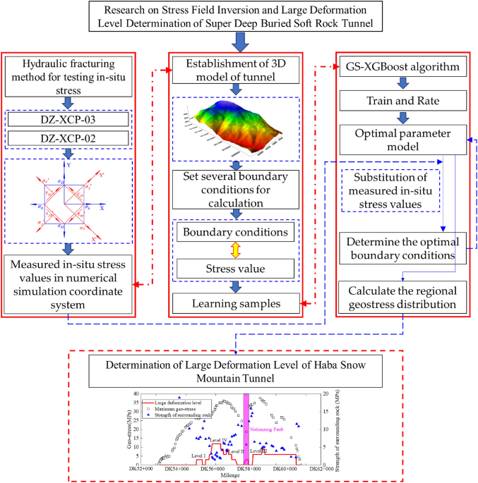
first tests the ground stress of the tunnel using the hydraulic fracturing method. Secondly, through numerical simulation methods combined with the GS-XGBoost algorithm, the in-situ stress

field of the tunnel site is inverted. Combined with the on-site in-situ stress test results, the effectiveness of the numerical model's in-situ stress inversion information is verified,

and the numerical values and characteristics of the tunnel site's in-situ stress are obtained. Then, the distribution pattern of ground stress in the longitudinal direction of the

tunnel will be analyzed. Finally, the level of large deformation of the Haba Snow Mountain Tunnel will be determined. The technical roadmap for this study is shown in Fig. 1. GROUND STRESS

FIELD INVERSION THEORY FACTORS AFFECTING THE GEO-STRESS FIELD For general geological bodies, the geo-stress field mainly considers the influence of the self weight of surrounding rock and

tectonic movement28. The self weight of the surrounding rock is mainly influenced by the density of the rock mass and the local gravitational acceleration, and tectonic movement is mainly

reflected in compression and shear29. Previous studies have shown no necessary connection between horizontal principal stress and vertical stress in rock masses. The lateral pressure

coefficient is not the same in different directions, and the horizontal principal stress is mainly related to geological tectonic movement30. From practical engineering experience, it can be

inferred that the gravity of the rock mass itself and the geological tectonic process are the main factors affecting the initial geo-stress31. Therefore, this geo-stress inversion mainly

considers the basic influencing factors of the initial geo-stress field, including ① Self-weight stress: The results of in-situ stress testing and a large number of practical engineering

geo-stress regression studies have shown that self weight stress is one of the main causes of the formation of rock mass geo-stress field. ② Horizontal uniform compression tectonic movement

in the east–west X-direction (see Fig. 2a). ③ Horizontal uniform compression tectonic movement in the north–south Y-direction (see Fig. 2b). ④ Shear deformation tectonic movement (see Fig.

2c). HYDRAULIC FRACTURING METHOD The hydraulic fracturing method testing is based on elastic mechanics with three assumptions as prerequisites: ① The rock is linearly elastic and isotropic.

② The rock is intact, and the fracturing fluid is impervious to the rock. ③ The vertical stress direction of the rock layer is parallel to the drilling axis. Obtain the in-situ stress value

of the measuring point by injecting water and pressurizing32. Figure 3 shows the stress distribution in the rock mass containing boreholes _σ_H is the maximum horizontal principal stress,

_σ_h is the minimum horizontal principal stress33. By substituting the stress state of element M in Fig. 3 into the wall of the circular hole, the stress state at any point on the wall of

the circular hole can be obtained, as shown in Eq. (1). $$\left\{ \begin{gathered} \sigma_{r} = 0 \hfill \\ \sigma_{\theta } = \left( {\sigma_{H} + \sigma_{h} } \right) - \left( {2\sigma_{H}

- \sigma_{h} } \right)\cos 2\theta \hfill \\ \tau_{r\theta } = 0 \hfill \\ \end{gathered} \right.$$ (1) In Eq. (1), _σ_r and _σ_θ, The radial and tangential stress on the hole wall are

represented, respectively. According to Eq. (1), the stress Eq. (2) for four points _A_、_A'_、_B_ and _B'_ on the circular hole wall can be obtained. Based on this Equation, the

in-situ stress value of the measurement point can be obtained by substituting multiple injection pressures. $$\left\{ \begin{gathered} \sigma_{A} = \sigma_{{A^{\prime}}} = 3\sigma_{h} -

\sigma_{H} \hfill \\ \sigma_{B} = \sigma_{{B^{\prime}}} = 3\sigma_{H} - \sigma_{h} \hfill \\ \end{gathered} \right.$$ (2) During the testing process, for the first time, water is injected

and pressurized to the critical rupture pressure _P_b in the dividing section. Suppose the critical rupture water pressure at the measuring point is greater than the ultimate tensile

strength Thf of the rock. In that case, tensile rupture will occur along the minimum tangential stress position _A_ and the symmetric point _A'_. It will propagate along the direction

of the vertical minimum principal stress. Considering the pore pressure _P_0 within the rock, the stress relationship can be expressed as Eq. (3). $$P_{b} = 3\sigma_{h} - \sigma_{H} + T_{hf}

- P_{0}$$ (3) After the hole wall ruptures, continue injecting water and pressurize; the crack will further expand towards deeper layers. Ensure that the fracturing circuit is sealed, that

water injection is stopped, and that the cracks will close under geo-stress. At this point, the equilibrium pressure at the critical closure state of the crack is the instantaneous closure

pressure _P_s, equal to the minimum horizontal principal stress measured in the borehole. $$\sigma_{h} = P_{s}$$ (4) After injecting water and pressurizing the test partition section again,

the crack reopened. As the rock had already ruptured at this time, the tensile strength _T__hf_ was 0. Based on the relationship between the critical fracture pressure, re-tension pressure,

and instantaneous closure pressure of the crack, the maximum horizontal principal stress calculation Eq. (5) can be obtained by substituting it into Eq. (3), where _P_r is the again open

pressure of the crack. $$\sigma_{H} = 3P_{s} - P_{r} - P_{0}$$ (5) According to the aforementioned assumption ③, the vertical stress _σ_v is equal to the self-weight of the soil cover. Thus,

the magnitude of the geo-stress in the separation section of the hydraulic fracturing test hole can be obtained. GS-XGBOOST ALGORITHM GS (Grid Search) is an exhaustive parameter tuning

method34. Among all the candidate parameters, adjust the parameters in order of step size and try every possibility through loop traversal to find the parameter with the highest accuracy on

the validation set from all the parameters. The best performing parameter is the final result. Grid search can ensure that the most accurate parameter is found within the specified parameter

range, as it traverses all possible combinations of parameters34. The principle of GS-XGBoost Algorithm is shown in Fig. 4. The principle of Grid Search is shown in Fig. 4a, and the

principle of XGBoost Algorithm is shown in Fig. 4b. The XGBoost algorithm improves the Gradient Ascension Decision Tree Theory (GBDT). The XGBoost algorithm and Gradient Boosting Decision

Tree Theory (GBDT) are ensemble learning methods based on Boosting thinking35. Gradient Boost Decision Tree Theory (GBDT) only uses first-order derivatives for optimization, while the

XGBoost algorithm performs second-order Taylor expansion on the function, using both first-order and second-order derivatives. Therefore, the XGBoost algorithm has advantages such as high

accuracy, fast running speed, the ability to process large-scale data, and the ability to customize objective functions. The XGBoost algorithm is an integrated algorithm that uses

classification and regression trees as the basic models. In XGBoost, the predicted value of the sample is the sum of the predicted values of each tree in _K_ trees. Define the function as:

$$\hat{y}^{(k)} = \sum\limits_{k = 1}^{K} {f_{k} } \left( {x_{i} } \right)$$ (6) Among them, _f_k is the k-th decision tree. _x_i is the characteristic value corresponding to sample _i.

f_k(_x_i) is the leaf weight, which denotes the predicted value of the k-th tree for sample _i_. The prediction result of XGBoost is the sum of the leaf weight weights of _K_ trees. The

objective function of the XGBoost algorithm is: $$L(\emptyset ) = \sum\limits_{i = 1}^{n} l \left( {y_{i} ,\hat{y}_{i} } \right) + \sum\limits_{k = 1}^{K} \Omega \left( {f_{k} } \right)$$

(7) This loss function consists of two components: the loss value \(\sum l \left( {y_{i} ,\hat{y}_{i} } \right)\) and the regularization term \(\Omega \left( {f_{k} } \right)\), in which the

loss value measures the difference between the true label _y_i and the predicted value \(\hat{y}_{i}\), and the regularization term controls the complexity of the model. The residuals of

the last prediction need to be fitted to the tree generated each time; i.e., when a tree is generated, the predicted values are: $$\hat{y}^{(t)} = \sum\limits_{k = 1}^{t} {f_{k} } \left(

{x_{i} } \right) = \hat{y}^{(t + 1)} + f_{t} \left( {x_{i} } \right)$$ (8) Therefore, the objective function can be rewritten as: $$L^{(t)} = \Omega \left( {f_{t} } \right) + \sum\limits_{i

= 1}^{n} l \left( {y_{i}^{t} ,\hat{y}^{(t + 1)} + f_{t} \left( {x_{i} } \right)} \right)$$ (9) The next step is to find _f_t, which is the minimization of the objective function. The

second-order Taylor expansion of the objective function is as follows: $$L^{(t)} = \Omega \left( {f_{t} } \right) + \sum\limits_{i = 1}^{n} {\left[ {l\left( {y_{i}^{t} ,\hat{y}^{(t + 1)} +

\frac{1}{2}h_{i} f_{t}^{2} \left( {x_{i} } \right) + g_{i} f_{t} \left( {x_{i} } \right)} \right)} \right]}$$ (10) where _g_i is the first derivative and _h_i is the second derivative:

$$g_{i} = \partial_{{\hat{y}^{(t - 1)} }} l\left( {y_{i} ,\hat{y}_{i}^{(t - 1)} } \right),h_{i} = \partial_{{\hat{y}^{(t - 1)} }}^{2} l\left( {y_{i} ,\hat{y}_{i}^{(t - 1)} } \right)$$ (11)

The predicted value of the (t − 1) th tree and the residual of y do not affect the optimization of the objective function and can be directly deleted. Therefore, the objective function is

simplified as: $$L^{(t)} = \Omega \left( {f_{t} } \right) + \sum\limits_{i = 1}^{n} {\left[ {f_{t} \left( {x_{i} } \right)g_{i} + \frac{1}{2}f_{t}^{2} \left( {x_{i} } \right)h_{i} }

\right]}$$ (12) The regularization term \(\Omega \left( {f_{t} } \right)\) is: $$\Omega \left( {f_{t} } \right) = \gamma T + \frac{1}{2}\lambda \left\| { \cdot \omega } \right\|^{2} = \gamma

T + \frac{1}{2}\lambda \sum\limits_{j = 1}^{T} {\omega_{j}^{2} }$$ (13) where _T_ is the number of leaf nodes and \(\omega_{j}^{{\phantom{0}}}\) represents the predicted value of the _j-_th

leaf node. After substituting the objective function: $$\begin{gathered} L^{\left( t \right)} = \sum\limits_{i = 1}^{n} {\left[ {g_{i} f_{t} \left( {x_{i} } \right) + \frac{1}{2}h_{i}

f_{t}^{2} \left( {x_{i} } \right)} \right]} + \Omega \left( {f_{t} } \right) \hfill \\ = \sum\limits_{i = 1}^{n} {\left[ {g_{i} \omega_{{q\left( {x_{i} } \right)}} + \frac{1}{2}h_{i}

\omega_{{q\left( {x_{i} } \right)}}^{2} } \right]} + \gamma T + \lambda \frac{1}{2}\sum\limits_{J = 1}^{T} {\omega_{J}^{2} } \hfill \\ = \sum\limits_{j = 1}^{T} {\left[ {\left(

{\sum\limits_{{i \in I_{j} }} {g_{i} } } \right)\omega_{j} + \frac{1}{2}\left( {\sum\limits_{{i \in I_{j} }} {h_{j} } + \lambda } \right)\omega_{j}^{2} } \right]} + \gamma T \hfill \\

\end{gathered}$$ (14) where _T_ is the number of leaf nodes in the decision tree _f_t, and _I__j_ represents the combination of all sample indexes belonging to leaf node _j._ Let \(G_{j} =

\sum {_{i \in I_{j}} } g_{i}\), \(H_{j} = \sum {_{i \in I_{j} } } h_{i}\), the objective function is then $$L^{(t)} = \left[ {\sum\limits_{i = 1}^{n} {G_{j} } \omega_{j} + \frac{1}{2}\left(

{H_{j} + \lambda } \right)\omega_{j}^{2} } \right] + \gamma T$$ (15) Assuming that the structure of the decision tree is known, and by setting the derivative of the objective function

relative to \(\omega_{j}^{{\phantom{0}}}\) be 0, the prediction on each leaf node can be obtained under the condition of minimizing the loss function as $$\omega_{j}^{*} = - \frac{{G_{j}

}}{{H_{j} + \lambda }}$$ (16) The minimum value of the loss function can be found by bringing the predicted values into it: $$L_{j}^{*} = - \frac{1}{2}\sum\limits_{j = 1}^{T}

{\frac{{G_{j}^{2} }}{{H_{j} + \lambda }}} + \gamma T$$ (17) It is easy to calculate the difference of the loss function before and after splitting: $${\text{ Gain }} = \frac{{G_{L}^{2}

}}{{H_{L} + \lambda }} + \frac{{G_{R}^{2} }}{{H_{R} + \lambda }} - \frac{{\left( {G_{L} + G_{R} } \right)^{2} }}{{H_{L} + H_{R} + \lambda }} - \gamma$$ (18) XGBoost constructs the decision

tree based on the difference obtained from Eq. (18), and by traversing the value cases of all features, a node is selected for splitting when the difference between the value before and

after the loss function reaches the maximum value. In addition, the difference in the loss function before and after splitting must be positive, which can be considered to play the role of

prehearing. INVERSION PROCESS OF IN-SITU STRESS FIELD The specific process of in-situ stress field inversion is shown in Fig. 5. ① Conduct data research and on-site investigation to obtain

basic information such as topographic maps, borehole histograms, structural distribution, and physical properties of rock layers. Use mapping software to establish a three-dimensional

geological model. ② Import the geological model into the finite element calculation software and establish a three-dimensional finite element calculation model through steps such as material

parameter definition and mesh division. Then, based on the comprehensive influencing factors of the geo-stress field, several sets of boundary condition combinations are set up and applied

to the finite element model for stress calculation. ③ Obtain the simulated stress magnitude of the measured point positions, establish corresponding relationships between the stress states

and boundary conditions at all positions, and create learning samples. ④ Write a GS-XGBoost regression algorithm model using Python, train and score the learning samples into the model,

adjust the model parameters based on the score, and find the optimal parameter model. ⑤ Substitute the measured in-situ stress values into the optimal parameter model and obtain the

predicted values as the corresponding optimal boundary conditions. ⑥ Substitute the optimal boundary condition parameters into the three-dimensional finite element calculation model for

stress solution and obtain the distribution of the in-situ stress field of the entire calculation model. INVERSION OF GROUND STRESS FIELD IN HABA SNOW MOUNTAIN TUNNEL ESTABLISHMENT OF A

THREE-DIMENSIONAL MODEL FOR THE HABA SNOW MOUNTAIN TUNNEL By using numerical simulation methods to invert the geo-stress field in the tunnel site area and combining with the results of

on-site geo-stress drilling tests, the effectiveness of the numerical model's geo-stress inversion information is verified, and the distribution pattern of longitudinal geo-stress in

the tunnel is obtained. The research area mainly focuses on the rectangular range of the entire Haba Snow Mountain Tunnel, as shown in Fig. 6a, with longitude of

100.039605680°–100.090074125° and latitude of 27.177790207°–27.256411118°. Tunnel entrance coordinates (E607800, N3008000), exit coordinates (E603244, N3016375). Obtain satellite images of

the tunnel surface through the 91 satellite map assistant, use the "elevation download" function to frame the research area, use the 15th level elevation, sampling distance of

67.97 m, select the "Xi'an 80 coordinate system Gaussian projection" for coordinate projection, and save it as a Surfer grid file. Using the contour drawing function in Surfer

software, plot the elevation information in the 91 satellite map assistant, as shown in Fig. 6b. The horizontal and vertical coordinates in the figure are the local coordinate system

automatically generated by Surfer software, and the red thick lines represent the tunnel position. Further, the elevation information is processed, and the three-dimensional transformation

is performed, with the surface elevation shown in Fig. 6c. Export the contour lines processed in Surfer software to a dxf format file, and use Rhino software to process the dxf file. Divide

the contour lines within the study area into points (curve → point object → segment length), with a division size of 50 m, and generate surface point information as shown in Fig. 7a. Based

on point information, generate a mesh and apply MeshPatch to the mesh, as shown in Fig. 7b. The line extrusion surface command and the cover command in entity extension generate a solid

model, as shown in Fig. 7c. Grid the solid model and export the model information through the Griddle plugin in Rhino. Import the model into FLAC3D and generate the research area model, as

shown in Fig. 7d. The model is 7850 m long and 4730 m wide. Assigning different parameters and constitutive relationships to different strata in the model and conducting calculations.

According to tunnel excavation, the rock mass joints are relatively dense. Therefore, to consider the influence of joints on the stability of surrounding rock and the stress of support, this

article adopts the Bilinear Strain Softening ubiquitous Joint Model in FLAC3D, hereinafter referred to as the Bilinear Model36,37. Based on the structural plane information obtained on site

(Table 1) and engineering experience analogy, the recommended values of rock and fault physical and mechanical parameter indicators in the tunnel site area are shown in Table 2. OPTIMAL

BOUNDARY CONDITION PREDICTION AND IN-SITU STRESS INVERSION BASED ON GS-XGBOOST ALGORITHM The in-situ stress values were obtained through the hydraulic fracturing method, and two deep holes

(DZ-XCP-02 and DZ-XCP-03) in the middle of the tunnel were subjected to in-situ stress testing. The elevation of borehole DZ-XCP-02 is 2750.01 m, located at DK54 + 310, and the tunnel is

buried at a depth of approximately 700 m. The elevation of drilling hole DZ-XCP-03 is 3007.70 m, and the buried depth of the tunnel here is 861.5 m, corresponding to the tunnel stake number

DK55 + 606.20. The drilling position is shown in Fig. 12. The results of in-situ stress measurement are shown in Tables 3 and 4. The depth of borehole DZ-XCP-02 is relatively shallow, and

the maximum and minimum horizontal ground stresses buried at depths of 700–1155 m are relatively large, mainly influenced by surface erosion. The erosion process shapes the terrain and

topography of the surface, thereby affecting the release and accumulation of local geological stress. The maximum depth of borehole DZ-XCP-03 is 888.70 m, which has good reference value. The

average fracture angle of the test results is N 26°–62° W, with an average value of N44° W. The coordinate system used for calculating the three-dimensional model is generally different

from the coordinate system used for calculating the measured in-situ stress. Therefore, coordinate transformation is necessary to determine the maximum horizontal principal stress, minimum

horizontal principal stress, and vertical stress directions38. Based on existing in-situ stress information, after screening, it has been determined that this article's measured data

used for in-situ stress inversion are measurement points 2, 4, and 6 in borehole DZ-XCP-03. The coordinate system used for the measured ground stress mentioned in this article is a natural

coordinate system, which has an angle with the direction of the tunnel axis. Therefore, it is necessary to consider this angle to convert the measured ground stress into the applicable

ground stress value in the model. In Fig. 8, XY is the coordinate system used for measurement, while XʹYʹ is the model coordinate system. The transformation relationship of the principal

stress during the transformation from the measurement coordinate system to the model coordinate system is determined by Eq. (19). $$\left\{ {\begin{array}{*{20}l} {\sigma_{x}^{\prime } =

\sigma_{x} l_{1}^{2} + \sigma_{y} m_{1}^{2} + 2\tau_{yx} l_{1} m_{1} } \hfill \\ {\sigma_{y}^{\prime } = \sigma_{x} l_{2}^{2} + \sigma_{y} m_{2}^{2} + 2\tau_{yx} l_{2} m_{2} } \hfill \\

{\tau_{xy}^{\prime } = \sigma_{x} l_{1} l_{2} + \sigma_{y} m_{1} m_{2} + 2\tau_{yx} \left( {l_{1} m_{2} + l_{2} m_{1} } \right)} \hfill \\ \end{array} } \right.$$ (19) In the Equation:

\(\sigma_{x}\), \(\sigma_{y}\), \(\tau_{yx}\) represents the stress values of each item in the initial coordinate system. \(\sigma_{x}^{\prime }\), \(\sigma_{y}^{\prime }\),

\(\tau_{xy}^{\prime }\) is the stress value after being converted to the new coordinate system. \(l_{1}\), \(l_{2}\), \(m_{1}\), \(m_{2}\) is the cosine of the direction corresponding to

each coordinate axis in the old and new coordinate systems. \(\alpha\) is the rotation angle of the old coordinate system in a counterclockwise direction. For the calculation coordinate

system of the Haba Snow Mountain Tunnel model, it is known from the characteristics of the regional stress field that \(\sigma_{y} { = }\sigma_{H}\), \(\sigma_{x} { = }\sigma_{h}\), \(\alpha

= 44^\circ\). The relationship between \(\sigma_{x}^{\prime }\), \(\sigma_{y}^{\prime }\), \(\tau_{xy}^{\prime }\) in the calculated coordinate system and the measured stress is shown in

Eq. 15. $$\left\{ {\begin{array}{*{20}l} {\sigma_{x}^{\prime } = \sigma_{h} \cos^{2} (44^{^\circ } ) + \sigma_{H} \sin^{2} (44^{^\circ } )} \hfill \\ {\sigma_{y}^{\prime } = \sigma_{h}

\sin^{2} (44^{^\circ } ) + \sigma_{H} \cos^{2} (44^{^\circ } )} \hfill \\ {\tau_{xy}^{\prime } = \left( {\sigma_{h} + \sigma_{H} } \right)\sin (44^{^\circ } )\cos (44^{^\circ } )} \hfill \\

\end{array} } \right.$$ (20) The above borehole geo-stress information is converted through coordinate transformation into the tunnel model coordinate system. Figure 8 is a schematic diagram

of stress direction transformation, and the transformed geo-stress information is shown in Table 5. From Table 5, it can be seen that for the coordinate system of the geo-stress inversion

model, the range of horizontal lateral pressure coefficients is \(\lambda_{X}\) = 0.76–0.96, \(\lambda_{Y}\) = 0.88–1.15, and the range of shear stress in the XY direction is \(\tau_{XY}\) =

 − 15.66 to − 19.79 MPa. Based on the measured values of the weight of the surrounding rock under in-situ stress and the actual weight of the surrounding rock, it can be concluded that the

weight compensation value \(\lambda_{G}\) = 1.11–1.33. Therefore, different boundary conditions are designed as shown in Table 6, and the optimal boundary conditions are obtained through the

GS-XGBoost algorithm as shown in Table 7, with \(\lambda_{G}\) = 1.23, \(\lambda_{X}\) = 0.94, \(\lambda_{Y}\) = 1.12, \(\tau_{XY}\) = 18.21 MPa. The results of in-situ stress inversion are

shown in Table 8. Table 8 shows that the difference between the inversion results of ground stress and the measured results is between − 15 and 19%, which can, to some extent, restore the

distribution of the ground stress field in the tunnel area. The difference may be because the lithology and geological structure of the tunnel area cannot be obtained through a small amount

of drilling, and the distribution of the lithology and geological structure is relatively complex. Only the main strata and structures were considered in the simulation. ANALYSIS OF

INVERSION RESULTS OF GROUND STRESS FIELD The geo-stress information on the tunnel axis is extracted by inverting the geo-stress field in the tunnel area. After coordinate transformation, it

is shown in Figs. 9 and 10. From Figs. 9 and 10, it can be seen that the tunnel ground stress increases with the increase of burial depth, with the maximum horizontal ground stress of 38.03 

MPa and the maximum, minimum horizontal ground stress of 26.07 MPa, located near the tunnel section DK58 + 877. In addition, according to the in-situ stress information, the pattern of the

in-situ stress field near the fault is that the in-situ stress on the upper wall of the fault increases, and the in-situ stress on the lower wall decreases. DETERMINATION OF LARGE

DEFORMATION LEVEL OF HABA SNOW MOUNTAIN TUNNEL Haba Snow Mountain is located on the southeast edge of the Qinghai Tibet Plateau, in the middle section of the Hengduan Mountains, on the left

bank of the Jinsha River, and belongs to the plateau tectonic erosion landform area39. The mountain runs in a nearly north–south direction, with a terrain low on the left and high on the

right, and is located in the eroded platform of the Chongjiang River and Jinsha River. The ground elevation ranges from 2050 to 3400 m, with significant terrain fluctuations and a natural

cross slope of 15°–40°, with local cliffs. The Haba Snow Mountain Tunnel is a mountain crossing tunnel with well-developed vegetation on the slope, mostly pine forests. The tunnel site area

only has soil access roads that can reach the entrance and exit of the tunnel, and most of the transverse tunnel exits are transported on average. The total length of the tunnel is 9523 m,

with the maximum burial depth (1155 m) at the tunnel mileage of approximately DK58 + 900. The surrounding rock of the tunnel is mainly composed of schistose basalt and sandy slate. The basic

engineering information of the Haba Snow Mountain Tunnel is shown in Fig. 11, and the geological profile is shown in Fig. 12. The classification of large deformation of Haba Snow Mountain

Tunnel adopts the classification standard for the deformation grade of compressible surrounding rock tunnels. This classification method mainly considers the strength and stress ratio of the

rock mass (_G_N), as shown in Table 9. According to the on-site testing results of severe large deformation sections, the rock mass strength of the Haba Snow Mountain Tunnel is 1.3–3.7 MPa.

According to the inversion results of ground stress, the tunnel ground stress is about 26.07–38.03 MPa. Therefore, the rock mass strength stress ratio of the severe large deformation

section of the tunnel is 0.03–0.09, belonging to level IV soft rock large deformation. Other paragraphs have significant deformations of levels I, II, and III. Therefore, the determination

of the large deformation level of the Haba Snow Mountain Tunnel is shown in Fig. 13. Figure 13 shows that the Haba Snow Mountain Tunnel has large deformation problems of Levels I, II, III,

and IV. The maximum in-situ stress in the Level I large deformation section is between 18.71 and 34.17 MPa, and the strength of the surrounding rock is between 5.78 and 10.29 MPa. The

maximum in-situ stress in the Level II large deformation section is between 11.08 and 37.76 MPa, and the strength of the surrounding rock is between 2.21 and 6.54 MPa. The maximum in-situ

stress in the Level III large deformation section is between 28.52 and 36.47 MPa, and the strength of the surrounding rock is between 3.23 and 5.11 MPa. The maximum in-situ stress in the

Level IV large deformation section is between 28.70 and 35.14 MPa, and the strength of the surrounding rock is between 1.55 and 3.48 MPa, mainly concentrated near DK56 + 000. Level III and

IV large deformations are generally accompanied by higher ground stress (above 28 MPa) and smaller surrounding rock strength (below 6.0 MPa). The distribution of surrounding rock strength in

the direction of the tunnel axis shows a clear "W" shape, opposite to the surface elevation "M" shape. Based on the Haba Snow Mountain Tunnel's terrain on the banks

of the Jinshan River, it is inferred that the mountain may be affected by geological structures on both sides, causing more severe compression of the tunnel surrounding rock at the mountain

peak. CONCLUSION Based on the GS-XGBoost Algorithm, the inversion of the ground stress in the Haba Snow Mountain Tunnel shows that the difference between the inversion results and the

measured results is − 15 to 19%, which can to some extent restore the distribution of the ground stress field in the tunnel area. The tunnel ground stress increases with burial depth, with a

maximum horizontal ground stress of 38.03 MPa and a minimum horizontal ground stress of 26.07 MPa, located near the tunnel section DK58 + 877. The Haba Snow Mountain Tunnel has large

deformation problems of Level I, II, III, and IV. Level III and IV large deformations are generally accompanied by higher ground stress (above 28 MPa) and smaller surrounding rock strength

(below 6.0 MPa). The distribution of surrounding rock strength in the direction of the tunnel axis shows a clear "W" shape, opposite to the surface elevation "M" shape.

Based on the Haba Snow Mountain Tunnel's terrain on the banks of the Jinshan River, it is inferred that the mountain may be affected by geological structures on both sides, causing more

severe compression of the tunnel surrounding rock at the mountain peak. The trend of combining intelligent algorithms with in-situ stress inversion methods is evolving. However, further

research is needed on the accuracy of the inversion of in-situ stress field range and the density of in-situ stress measured boreholes. In addition, the impact of the accuracy of in-situ

stress testing methods on the results of in-situ stress inversion is also worth further exploration. DATA AVAILABILITY The datasets used and analyzed during the current study are available

from the corresponding author upon reasonable request. REFERENCES * Zhao, C. _et al._ Asymmetric large deformation of tunnel induced by groundwater in carbonaceous shale. _Bull. Eng. Geol.

Environ._ 81, 260 (2022). Article  Google Scholar  * Zhao, J., Tan, Z., Li, Q. & Li, L. Characteristics and mechanism of large deformation of squeezing tunnel in phyllite stratum. _Can.

Geotech. J._ 61, 59–74 (2023). Article  Google Scholar  * Deng, H.-S., Fu, H.-L., Shi, Y., Zhao, Y.-Y. & Hou, W.-Z. Countermeasures against large deformation of deep-buried soft rock

tunnels in areas with high geostress: A case study. _Tunn. Undergr. Space Technol._ 119, 104238 (2022). Article  Google Scholar  * Wu, K. _et al._ Determination of stiffness of

circumferential yielding lining considering the shotcrete hardening property. _Rock Mech. Rock Eng._ 56, 3023–3036 (2023). Article  ADS  Google Scholar  * Lu, A. _et al._ Numerical

simulation on energy concentration and release process of strain rockburst. _KSCE J. Civ. Eng._ 25, 3835–3842 (2021). Article  Google Scholar  * Li, J., Wang, Z.-F., Wang, Y. & Chang, H.

Analysis and countermeasures of large deformation of deep-buried tunnel excavated in layered rock strata: A case study. _Eng. Fail. Anal._ 146, 107057 (2023). Article  Google Scholar  *

Sun, Z. _et al._ Support countermeasures for large deformation in a deep tunnel in layered shale with high geostresses. _Rock Mech. Rock Eng._ 56, 4463–4484 (2023). Article  ADS  Google

Scholar  * Jin, D., Ng, Y. C. H., Han, B. & Yuan, D. Modeling hydraulic fracturing and blow-out failure of tunnel face during shield tunneling in soft soils. _Int. J. Geomech._ 22,

06021041 (2022). Article  Google Scholar  * Zhou, P. _et al._ Stability evaluation method and support structure optimization of weak and fractured slate tunnel. _Rock Mech. Rock Eng._ 55,

6425–6444 (2022). Article  ADS  Google Scholar  * Krietsch, H. _et al._ Stress measurements for an in situ stimulation experiment in crystalline rock: integration of induced seismicity,

stress relief and hydraulic methods. _Rock Mech. Rock Eng._ 52, 517–542 (2019). Article  ADS  Google Scholar  * Zhao, J., Tan, Z., Li, L. & Wang, X. Supporting structure failure caused

by the squeezing tunnel creep and its reinforcement measure. _J. Mt. Sci._ 20, 1774–1789 (2023). Article  Google Scholar  * Liu, X., Liu, F. & Song, K. Mechanism analysis of tunnel

collapse in a soft-hard interbedded surrounding rock mass: A case study of the Yangshan Tunnel in China. _Eng. Fail. Anal._ 138, 106304 (2022). Article  MathSciNet  Google Scholar  * Tan,

Z., Li, S., Yang, Y. & Wang, J. Large deformation characteristics and controlling measures of steeply inclined and layered soft rock of tunnels in plate suture zones. _Eng. Fail. Anal._

131, 105831 (2022). Article  Google Scholar  * Chen, Z. _et al._ Stability analysis and deformation control of tunnel with extremely weak surrounding rocks caused by strike-slip fault

activity. _Rock Mech. Rock Eng._ 56, 8543–8569 (2023). Article  ADS  Google Scholar  * Song, Z., Yang, Z., Huo, R. & Zhang, Y. Inversion analysis method for tunnel and underground space

engineering: A short review. _Appl. Sci._ 13, 5454 (2023). Article  CAS  Google Scholar  * Cai, W. _et al._ Three-dimensional forward analysis and real-time design of deep tunneling based on

digital in-situ testing. _Int. J. Mech. Sci._ 226, 107385 (2022). Article  Google Scholar  * Sharifzadeh, M., Tarifard, A. & Moridi, M. A. Time-dependent behavior of tunnel lining in

weak rock mass based on displacement back analysis method. _Tunn. Undergr. Space Technol._ 38, 348–356 (2013). Article  Google Scholar  * Zhou, Z. _et al._ Study on the applicability of

various in-situ stress inversion methods and their application on sinistral strike-slip faults. _Rock Mech. Rock Eng._ 56, 3093–3113 (2023). Article  ADS  Google Scholar  * Chu, Z. _et al._

Viscos-elastic-plastic solution for deep buried tunnels considering tunnel face effect and sequential installation of double linings. _Comput. Geotech._ 165, 105930 (2024). Article  Google

Scholar  * Yang, J., Sun, J., Jia, Y. & Yao, Y. Energy generation and attenuation of blast-induced seismic waves under in situ stress conditions. _Appl. Sci._ 12, 9146 (2022). Article 

CAS  Google Scholar  * Tan, N., Yang, R. & Tan, Z. Influence of complicated faults on the differentiation and accumulation of in-situ stress in deep rock mass. _Int. J. Miner. Metall.

Mater._ 30, 791–801 (2023). Article  Google Scholar  * Li, X., Jia, C., Zhu, X., Zhao, H. & Gao, J. Investigation on the deformation mechanism of the full-section tunnel excavation in

the complex geological environment based on the PSO-BP neural network. _Environ. Earth Sci._ 82, 326 (2023). Article  ADS  Google Scholar  * Yu, R., Tan, Z., Gao, J., Wang, X. & Zhao, J.

Inversion and analysis of the initial ground stress field of the deep-buried tunnel area. _Appl. Sci._ 12, 8986 (2022). Article  CAS  Google Scholar  * Du, E., Zhou, L. & Fei, R.

Investigation on the stress and deformation evolution laws of shield tunnelling through a mining tunnel structure. _Appl. Sci._ 13, 8489 (2023). Article  CAS  Google Scholar  * Zhang, K.,

Zhao, X. & Zhang, Z. Influences of tunnelling parameters in tunnel boring machine on stress and displacement characteristics of surrounding rocks. _Tunn. Undergr. Space Technol._ 137,

105129 (2023). Article  Google Scholar  * Xu, D., Hu, Q. & Si, H. Measurement and inversion of the stress distribution in a coal and rock mass with a fault. _Int. J. Geomech._ 21,

06021029 (2021). Article  Google Scholar  * Li, P., Cai, M., Miao, S. & Guo, Q. New insights into the current stress field around the Yishu fault zone, eastern China. _Rock Mech. Rock

Eng._ 52, 4133–4145 (2019). Article  ADS  Google Scholar  * Zhang, L. Q., Yue, Z. Q., Yang, Z. F., Qi, J. X. & Liu, F. C. A displacement-based back-analysis method for rock mass modulus

and horizontal in situ stress in tunneling–Illustrated with a case study. _Tunn. Undergr. Space Technol._ 21, 636–649 (2006). Article  ADS  Google Scholar  * Zhang, Z., Gong, R., Zhang, H.,

Lan, Q. & Tang, X. Initial ground stress field regression analysis and application in an extra-long tunnel in the western mountainous area of China. _Bull. Eng. Geol. Environ._ 80,

4603–4619 (2021). Article  Google Scholar  * Hao, X. _et al._ Effects of the major principal stress direction respect to the long axis of a tunnel on the tunnel stability: Physical model

tests and numerical simulation. _Tunn. Undergr. Space Technol._ 114, 103993 (2021). Article  Google Scholar  * Jiang, H. & Shi, K. Characterization of the high geostress field in

deep-buried diversion tunnels and its inversion analysis. in _2022 8th International Conference on Hydraulic and Civil Engineering: Deep Space Intelligent Development and Utilization Forum

(ICHCE)_ 301–310 (IEEE, 2022). * Piao, S., Huang, S., Wang, Q. & Ma, B. Experimental and numerical study of measuring in-situ stress in horizontal borehole by hydraulic fracturing

method. _Tunn. Undergr. Space Technol._ 141, 105363 (2023). Article  Google Scholar  * Luo, M.-R., Zhang, C.-Y., Wang, B. & Zeng, Y.-H. Discrete element-based regression analysis of

initial ground stress and application to an extra-long tunnel in China. _Bull. Eng. Geol. Environ._ 82, 405 (2023). Article  Google Scholar  * Feng, T., Wang, C., Zhang, J., Wang, B. &

Jin, Y.-F. An improved artificial bee colony-random forest (IABC-RF) model for predicting the tunnel deformation due to an adjacent foundation pit excavation. _Undergr. Space_ 7, 514–527

(2022). Article  Google Scholar  * Li, J.-B. _et al._ Feedback on a shared big dataset for intelligent TBM Part I: Feature extraction and machine learning methods. _Undergr. Space_ 11, 1–25

(2023). Article  Google Scholar  * Sardana, S., Sharma, P., Verma, A. K. & Singh, T. N. A case study on the rockfall assessment and stability analysis along Lengpui-Aizawl highway,

Mizoram. _India. Arab. J. Geosci._ 13, 1–12 (2020). Google Scholar  * Wang, Y., Liu, X. & Xiong, Y. Numerical simulation of zonal disintegration of surrounding rock in the deep-buried

chamber. _Deep Undergr. Sci. Eng._ 1, 174–182 (2022). Article  Google Scholar  * Jiang, Q. _et al._ Observe the temporal evolution of deep tunnel’s 3D deformation by 3D laser scanning in the

Jinchuan No. 2 Mine. _Tunn. Undergr. Space Technol._ 97, 103237 (2020). Article  Google Scholar  * Gong, Y., Yao, A., Li, Y., Li, Y. & Tian, T. Classification and distribution of

large-scale high-position landslides in southeastern edge of the Qinghai-Tibet Plateau, China. _Environ. Earth Sci._ 81, 311 (2022). Article  ADS  Google Scholar  Download references

ACKNOWLEDGEMENTS The authors thank the editors and reviewers for their efforts to improve the quality of the manuscript. The authors acknowledge the National Natural Science Foundation of

China (Grant no. 51978041). AUTHOR INFORMATION AUTHORS AND AFFILIATIONS * Key Laboratory of Urban Underground Engineering of Ministry of Education, Beijing Jiaotong University, Beijing,

100044, China Baojin Zhang, Zhongsheng Tan & Jinpeng Zhao * China Railway 16th Bureau Group 3rd Corporation Limited, Huzhou, 313000, China Fengxi Wang & Ke Lin * State Key Laboratory

of Hydroscience and Engineering, Tsinghua University, Beijing, 100084, China Jinpeng Zhao Authors * Baojin Zhang View author publications You can also search for this author inPubMed Google

Scholar * Zhongsheng Tan View author publications You can also search for this author inPubMed Google Scholar * Jinpeng Zhao View author publications You can also search for this author

inPubMed Google Scholar * Fengxi Wang View author publications You can also search for this author inPubMed Google Scholar * Ke Lin View author publications You can also search for this

author inPubMed Google Scholar CONTRIBUTIONS Baojin Zhang: Methodology, Data curation, Software, Visualization, Writing-review & editing. Zhongsheng Tan: Conceptualization, Methodology,

Funding acquisition, Supervision, Writing – review & editing. Jinpeng Zhao: Investigation, Data curation, Writing-original draft. Fengxi Wang: Writing – review & editing,

Supervision. Lin Ke: Data curation, Project administration. CORRESPONDING AUTHOR Correspondence to Jinpeng Zhao. ETHICS DECLARATIONS COMPETING INTERESTS The authors declare no competing

interests. ADDITIONAL INFORMATION PUBLISHER'S NOTE Springer Nature remains neutral with regard to jurisdictional claims in published maps and institutional affiliations. RIGHTS AND

PERMISSIONS OPEN ACCESS This article is licensed under a Creative Commons Attribution 4.0 International License, which permits use, sharing, adaptation, distribution and reproduction in any

medium or format, as long as you give appropriate credit to the original author(s) and the source, provide a link to the Creative Commons licence, and indicate if changes were made. The

images or other third party material in this article are included in the article's Creative Commons licence, unless indicated otherwise in a credit line to the material. If material is

not included in the article's Creative Commons licence and your intended use is not permitted by statutory regulation or exceeds the permitted use, you will need to obtain permission

directly from the copyright holder. To view a copy of this licence, visit http://creativecommons.org/licenses/by/4.0/. Reprints and permissions ABOUT THIS ARTICLE CITE THIS ARTICLE Zhang,

B., Tan, Z., Zhao, J. _et al._ Research on stress field inversion and large deformation level determination of super deep buried soft rock tunnel. _Sci Rep_ 14, 12739 (2024).

https://doi.org/10.1038/s41598-024-62597-9 Download citation * Received: 10 January 2024 * Accepted: 20 May 2024 * Published: 03 June 2024 * DOI: https://doi.org/10.1038/s41598-024-62597-9

SHARE THIS ARTICLE Anyone you share the following link with will be able to read this content: Get shareable link Sorry, a shareable link is not currently available for this article. Copy to

clipboard Provided by the Springer Nature SharedIt content-sharing initiative KEYWORDS * High geo-stress * Large deformation tunnel * GS-XGBoost algorithm * Geo-stress inversion * Large

deformation level