ABSTRACT The discovery and identification of geophysical features from diverse gridded datasets play a pivotal role in understanding geological phenomena. Traditional tools tailored to

identify specific signatures, such as lineaments in magnetic data, do not account for (1) the _naturally_ occurring complexity of the causative geology which results from competing and

overprinting processes and (2) often overlook important related patterns present in other forms of data (e.g., gradients in the associated gravity data). To address those limitations, we

propose a two-step data-driven approach that integrates diverse gridded datasets and autonomously reveals inherent patterns without predefined assumptions in terms of feature geometry.

atlas positions tiles from each dataset according to their position in the t-SNE while linking them back to their original geographical coordinates. Such a setup allows earth scientists to

intuitively navigate through the data, exploring complex relationships between geophysical responses and geological structures, thus facilitating the discovery of new insights, the

formulation of hypotheses, and the exploration of non-trivial connections. This is illustrated using magnetic and gravity data covering \(58,800 {\textrm{km}}^2\) in the east Yilgarn Craton,

Western Australia. Our methodology is adaptable and can be extended to include various other gridded datasets like gamma-ray spectrometry data, satellite imagery, and digital terrain

models, thus broadening its applicability and enhancing geoscientific exploration. Our approach not only reveals subtle geophysical patterns but also offers practical benefits for

exploration geologists. The atlas enables the identification of geological settings associated with mineral prospectivity and can serve as a pre-planning tool for pinpointing promising

exploration sites, potentially accelerating discovery timelines. SIMILAR CONTENT BEING VIEWED BY OTHERS CLASSIFYING SEISMOGRAMS USING THE FASTMAP ALGORITHM AND SUPPORT-VECTOR MACHINES

Article Open access 15 July 2023 PREDICTING ANCIENT CITY SITES USING GEE COUPLED WITH GEOGRAPHIC ELEMENT FEATURES AND TEMPORAL SPECTRAL FEATURES: A CASE STUDY OF THE NEOLITHIC AND BRONZE AGE

OF THE JIANGHAN REGION, CHINA Article Open access 11 February 2025 A NEW STRATEGY BASED ON MULTI-SOURCE REMOTE SENSING DATA FOR IMPROVING THE ACCURACY OF LAND USE/COVER CHANGE

CLASSIFICATION Article Open access 06 November 2024 INTRODUCTION Since the early days analysing digital images, researchers have tried to automatically extract meaning from them, both by

enhancing the images so that the information is more readily understood by the human eye and brain and by the automatic extraction of features from the images themselves1,2. With the release

of the first Landsat earthward looking satellite image of the Dallas Fort Worth area taken on July 25, 1972, earth scientists started to use digital data to interpret near-surface geology,

and all of the interpretive and automated tools developed over the previous decade were applied to these multi-band images3,4,5. In 1978 Huntington and Green, research scientists at the

Commonwealth Scientific and Industrial Research Organisation (CSIRO) applied the software developed process and analyse Landsat data to airborne geophysical data, and since that time there

has been a steady stream of researchers focused on extracting meaning from these gridded geophysical datasets in plan view6 and section view7,8,9,10. One of the drawbacks of using feature

extraction methods that search for _specific_ shapes (e.g., lineaments) in natural scenes such as geophysical data is that geological datasets are complex and do not follow simple rules, as

opposed to, e.g., face recognition. Indeed, human faces have a consistent and well-defined structure, with most faces having common features in predictable locations (e.g., two eyes

symmetrically located above one nose). This implies on a low-dimensional feature space with a simple structure, which enables the use of simple techniques like principal components analysis

(PCA) to capture the most significant features with fewer components11. In contrast, geological datasets are high-dimensional, exhibit irregular patterns with complex geophysical signatures,

and lack the same level of predictability and consistency, making feature extraction a (much) more challenging task12,13,14. Extracting meaningful features from such data often requires

sophisticated methods to manage the higher dimensionality and complexity of the feature space itself15,16,17,18,19,20,21,22,23. In this study, we propose a hybrid method that attempts to

cluster _naturally_ occurring geophysical features within small image patches and provide these clusters in a manner that allows the earth scientist to interpret these clustered images using

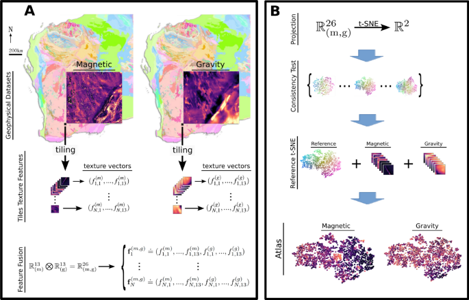
their prior knowledge of the region. The workflow is summarized in Fig. 1. Specifically, we explore the use of Haralick texture descriptors24,25,26,27 to encode the (high-dimensional)

patches and integrate diverse geophysical data into a cohesive lower dimensional space, and the t-distributed stochastic neighbor embedding (t-SNE)28,29,30,31 for the nonlinear projection in

2D to build a _t-SNE atlas_ for organizing multimodal geophysical information in a sensible way (see Methods for a detailed description). We also enhance this tool with interactive features

such as linking the t-SNE output to the _geographical locations_ of the original data and advocate its use as a dynamic tool for geophysical exploration, allowing a subject matter expert to

“navigate” large datasets in search of insights and meaning. The interactive tool is available at https://www.loopwms.xyz/wagravmag/. As one intermediary step, we also suggest a _perplexity

consistency_ test to select an optimal 2D embedding from a set of t-SNEs, thereby supporting more accurate interpretations and analyses of the data (see Methods). Our approach is

illustrated with magnetic and gravity data spanning \(58,800 \textrm{km}^2\) from the east Yilgarn Craton region in Western Australia. This is a geologically complex area, and a focal point

for mineral exploration, attracting considerable research and exploration efforts. The main novelties and advantages of our method are the ability to integrate diverse geophysical

information (i.e., data fusion through Haralick texture descriptors), its visualization and map navigation capabilities (i.e., 2D t-SNE projection, interactivity and link to geophysical

position), not too be limited by _specific_ shapes, and also its simplicity and rapidity. RESULTS Firstly, we carry out a perplexity consistency test on a set of embeddings to select one

that offers a balanced representation of both global and local structures, and also to ensure that it robustly maintains cluster integrity across different values of the hyperparameter

perplexity (see Methods). Figure 2.A shows the results using an embedding with perplexity \(\tau =40\) as the reference t-SNE for color mapping the points across all the other embeddings.

For the sake of space, results are shown for the range \(\tau \in (5, 60)\). Upon comparing the embeddings, one observes that the majority of points with similar colors are still neighbours,

therefore demonstrating a general consistency across the range of tested values. This consistency in cluster formation provides confidence in selecting a perplexity value of 40 as an

effective representation of the data in a lower-dimensional space, thereby capturing the intrinsic structure of the high-dimensional space effectively. Each map from the resulting t-SNE

atlas is shown in Fig 2.B-C. A visual inspection of this static representation indicates that similar features in geophysics will be observed in the same embedding location, as, for

instance, all of the 1663 gravity tiles are spread out in such a way that they form clusters of similar elements in terms of texture, and the same applies to the magnetic data. However, as

we will discuss later, a more careful investigation utilizing the interactive tool reveals the existence of a more nuanced structure (see the discussion of Region 2 from Fig. 4) The

implications of this arrangement are threefold. Firstly, it demonstrates that the use of texture descriptors for encoding, followed by feature fusion, provides a meaningful and consistent

representation of the geophysicalsignatures within the tiles. Secondly, the t-SNE embedding is effective in providing a comprehensible 2D representation of the cluster structure that occurs

in the 26D “Haralick-space”. Finally, it also reveals that the dataset itself contains a substantial number of samples (i.e., the tiles) with similar and diverse geophysics, which allows the

formation of clusters in the 26D space. This also supports the segmentation strategy applied to the geophysical images as tiles of size \(40\times 40\). A deeper analysis can be done by

utilizing the interactive visualization tool, available at https://www.loopwms.xyz/wagravmag/. Its capabilities are depicted in Figure 3. It allows the user to explore the t-SNE atlas by

moving back and forth between gravity and magnetic data, zooming in to examine different areas, select specific tiles and to map them back to the original geographical location (and

vice-versa). Therefore, the subject matter expert can utilize the interactive t-SNE atlas as a “navigation map”, facilitating the discovery of new insights, the formulation of hypotheses,

and the exploration of non-trivial connections among various geophysical data sets. To demonstrate this, we have highlighted three distinct regions within the t-SNE atlas, as depicted in

Fig. 4: * Region 1 – This region is characterized by a series of tiles with groups of parallel linear magnetic highs accompanied by a very smooth gravity gradient. Moreover, the steepest

gravity gradient is perpendicular to the orientation of the linear magnetic highs. These characteristics suggest that these particular tiles could correspond to areas with a dipping

stratigraphy. * Region 2 – A bright orange section in the middle of the magnetic data in t-SNE map (Fig. 2B) immediately draws one attention to this region. It consists of a series of tiles

dominated by linear and point magnetic lows, suggesting they are remnant dykes and other intrusions. Interestingly, there is no visually clear pattern in the associated gravity tiles,

indicating that this cluster in the data is largely influenced by the magnetic signal with those linear lows. * Region 3 – In this region the tiles are dominated by isolated linear magnetic

highs, which coincide with linear gravity highs. Thus, the geological phenomenon responsible for these features must possess both high density and significant magnetic susceptibility,

possibly representing a thicker stratigraphic package. In reality, several factors can cause linear gravity and magnetic highs, but this is where geologists step back into the picture. For

illustrative purposes, Fig. 5 shows the mapping between the image tiles from the t-SNE representation and their original geographical positions. The top panel shows some samples from the 3

aforementioned selected regions. The samples from regions 2 and 3 illustrate that the respective (integrated) geophysical signatures can be found in samples from very different geographical

locations, suggesting that the similar underlying geology might be found far apart from each other in the real-world coordinates. Conversely, the (integrated) geophysical features of the

samples from region 1 are related to complex sheared boundary of Biranup Zone and Northern Foreland on the western edge of the Fraser Zone within the Albany-Fraser Orogen35. Finally, the

bottom panel illustrates the overall structure seen in the t-SNE and its relationship with the original geographical positions by _blending_ the gray scale image of the geophysical datasets

with the the color code scheme from the reference t-SNE (see Methods). This approach not only demonstrates the correspondence between the geophysical data and the abstract clustering in

t-SNE but also provides an intuitive visual link between the two, thereby enhancing the interpretability of the spatial patterns observed. Emerging spatial patterns can prompt further

investigation to understand the relationship between the underlying geology and geophysical response. DISCUSSION In this study, we present a data-driven method for analyzing gridded

geophysical data that allows earth scientists to search for patterns in their datasets without preconceived notions of the specifics of these patterns. It also leverages the integration of

diverse gridded datasets, facilitated by the feature fusion of the Haralick texture descriptors, to autonomously reveal intrinsic patterns and significantly enhancing the interpretive

landscape for earth scientists. Thus, it allows one to discover _ naturally_ occurring patterns, as for instance the coincident linear highs, but also highlighting the commonalities in

geophysical response of remnant mafic dykes across the case study region. Of course these features can be explored for manually with a geographic information system (GIS); however previous

attempts to automate this process often result in too many false positives. This methodology has been demonstrated using magnetic and gravity data from the east Yilgarn Craton region in

Western Australia, showcasing its potential in a real-world setting. However, the versatility of our approach allows for its application to any gridded dataset, including gamma-ray

spectrometry data (radiometrics), satellite imagery, and digital terrain models. This adaptability opens the door for cross-disciplinary applications, potentially transforming how

geoscientists interact with and interpret gridded datasets. There are many possible extensions to this work. At the present time we only explore a fixed-size of image tiles, but

different-sized tiles could enable us to develop a multi-scale Atlas that highlights different relationships at different scales, and ensures that discrete features are captured at the

appropriate scale. It should be noticed, however, that the tile scale is crucial because it determines the level of detail captured from the geophysical data. Larger tiles tend to mix

multiple geological features, which can dilute the subtle textural variations that Haralick descriptors are designed to quantify. This mixing may lead to less distinct clusters in the t-SNE

projection. In contrast, if the tiles are too small, they might not contain enough spatial context to provide robust texture information, resulting in unstable or less meaningful descriptor

values. Additionally, overlapping tiles in a sliding window approach could prevent small geophysical anomalies being split across neighbouring tiles, therefore improving the continuity of

data interpretation. Our approach is also easily extensible to 3D datasets, and exploratory work is currently being undertaken to help us understand the outputs from stochastic inversion

codes for the rapid, streamlined analysis of 100’s of 1000’s of models in a single atlas representative of the search space. Finally, the feature parameterization (Haralick descriptors) and

2D projection (t-SNE) steps could be replaced by other techniques that fulfil similar goals (such as dissimilarity metrics17 and Multi-Dimensional Scaling or Uniform Manifold Approximation

and Projection, respectively). An interesting option for the featureparametrization is the use of the output from the intermediary layers of a convolutional neural network36. The strength of

the workflow presented here is that it is not based on prior assumptions of feature geometry and and integrates information from diverse gridded datasets, and thus can be used to navigate

single band or multi-band Earth Science data in a data-centric fashion, which allows one to discover patterns in grid data that may be missed by more conventional techniques. Specifically,

our approach is fundamentally data-driven because it abstains from predefined geological models or feature assumptions in favor of letting the data reveal its inherent structure. By fusing

Haralick texture descriptors into a unified high-dimensional feature space, an unbiased representation of the data is achieved, while the subsequent t-SNE dimensionality reduction highlights

natural clusters and relationships without imposing any prior interpretive framework. Consequently, the resulting visualization – the atlas – is a direct reflection of the underlying data

patterns and facilitates exploratory analysis that can be readily extended to additional gridded datasets. Our study offers practical applications that extend beyond simple clustering

analysis by providing valuable insights to geologists. For instance, our atlas can help exploration geologists identify specific geological settings and then assess the mineral prospectivity

of focused areas. By quantifying and visualizing subtle geophysical patterns, our tool provides a data-driven framework that can highlight areas of interest for focused exploration.

Additionally, the atlas can serve as a valuable pre-planning resource for exploration projects, enabling geologists to pinpoint promising locations to start their exploration journey which

could improve their discovery timeline. CONCLUSION In this work, we introduced a novel, data-driven methodology for the integrated interpretation of geophysical datasets. By encoding data

patches from both magnetic and gravity images using Haralick texture descriptors, we fused these complementary datasets into a unified 26-dimensional feature space. This integration allows

the t-SNE algorithm to simultaneously embed and visualize the combined geophysical signatures, thereby letting the inherent structure of the data to emerge and enhancing the resolution of

subtle geological features. When applied to the case study area, our approach successfully generates an interactive t-SNE atlas that not only reveals distinct clusters corresponding to

various geophysical patterns but also directly links these clusters back to their original geographic locations. This capability enables a more intuitive and comprehensive exploration of

complex geological structures, supporting both hypothesis generation and more targeted mineral exploration. To illustrate this, our analysis identified three distinct geophysical regions in

the t-SNE atlas that underscore the capability of our methodology to reveal complex geological patterns. The first region features clusters of tiles with parallel linear magnetic highs and a

smooth, perpendicularly oriented gravity gradient, suggesting dipping stratigraphy. The second region is characterized by a cluster dominated by linear and point magnetic lows – indicative

of remnant dykes and intrusions-with little corresponding gravity signal. This exemplifies a case where the subsurface configuration highlights the predominance of magnetic data for

inferring its properties. Finally, the third region exhibits isolated linear magnetic highs that align with linear gravity highs, suggesting a geological phenomenon with high density and

magnetic susceptibility, possibly a thicker stratigraphic unit. Overall, our methodology demonstrates significant added value by automating the identification of geological patterns, and

enabling a more objective, data-centric analysis of geophysical datasets. The unified feature space effectively integrates the information content from the magnetic and gravity datasets,

improving the robustness of geophysical interpretation compared to analyzing each dataset in isolation. It should be noticed that our method was _demonstrated_ using magnetic and gravity

data. However, encoding information through Haralick texture descriptors allows for data-fusion capability that makes it versatile and readily extendable to other gridded datasets, such as

gamma-ray spectrometry, satellite imagery, and digital terrain models. Consequently, we anticipate future applications incorporating a broader variety of data types. Future work will focus

on extending this framework to additional data types and scales, further enhancing its applicability across various geological settings. METHODS GEOLOGICAL SETTING AND DATA SET The

Palaeo-Neoarchean Yilgarn Craton in Western Australia has a long-lived and complex tectonic history and is subdivided into seven terranes37,38.The relevant part of our study is the Eastern

Goldfields Superterrane, which hosts substantial NNW-trending greenstone belts separated by granite and granitic gneiss. The greenstone belts are conspicuous in geophysical data, being

strong positive magnetic and gravity anomalies. The southeastern part of our study area is part of the Albany-Fraser Orogen which is separated into the Biranup, Fraser and Tropicana zones of

the Kepa Kurl Booya Province39 (Fig. 2). The 1815-1625 Ma Biranup Zone is dominated by strongly deformed orthogneiss and minor metagabbro and hybrid rocks39. The Fraser Zone is conspicuous

in potential field data with an anomalously high gravity and magnetic signature. The high-density rocks respond to the widespread occurrence of metagabbroic rocks40. The geological setting

is a large area from the east Yilgarn Craton region in Western Australia (WA), comprising a rectangular field with east-west (EW) dimension of \(840~\textrm{km}\) and the north-south (NS)

dimension of \(700~\textrm{km}\). To illustrate the method and its capabilities in integrating different types of gridded data, we selected the corresponding magnetic and gravity anomalies

of this area32,33. Figure 1.A shows the geophysical data overlaid on the geological map of WA. Each geophysical image is represented by a \(1826 \times 1512\) grid, with each grid cell

corresponding to an area of \(450~\textrm{m} \times 450~\textrm{m}\), with the magnetic data being upsampled to match the gravity data spatial resolution. TILING AND IMAGE ENHANCEMENT This

section describes the cropping and segmentation of the original magnetic and gravity images into small tiles and the subsequent re-scaling of the tiles grey scale levels. Firstly, the tiles

size for the segmentation of the grid must be selected. The guiding principle is that the t-SNE will group tiles with similar features in geophysics. If the tile size is too large, one incur

on the risk of having too many different and complex geophysical signatures within each tile, and specific local nuances will be lost. If the size is too small, there will be a lack of

information content to differentiate the tiles, or the lack of an actual signature that can be associated to geophysics. After careful visual inspection, we opted for square tiles of size

\(n\times n\), with \(n=40\) pixels, which provided a good balance between both scenarios. This corresponds to a physical area of dimensions \(18~\textrm{km} \times 18~\textrm{km}\). In

mineral exploration terms, this can be considered to be from camp to prospect scale, at a scale where important exploration decision need to be made in terms of the targeting of favourable

areas. In order to have an integer number of tiles, each image was cropped (in the east and in the north; see Supplementary Fig. 1 middle panel) resulting in a \(1800 \times 1480\) grid,

corresponding to (\(720~\textrm{km} \times 592~\textrm{km}\)). This resulted in \(N=1665\) tiles for each geophysical dataset. Due to the large difference in pixel intensity distribution,

some tiles appear almost flat (i.e., homogeneous; see Supplementary Fig. 1). To enhance the informationcontent, _each_ tile underwent amplitude normalization by re-scaling the pixel

intensities to (0, 255). Figure 1.A illustrates the process by showing the cropped images and the relative size of one tile indicated as a black square. All tiles are shown in the

Supplementary Fig. 1 bottom panel. In summary, the working data comprises a total of 3330 image tiles, grouped in two sets with 1665 images from each geophysical dataset: one for magnetic

data and the other for gravity data. Conceptually, the elements of each geophysical set are represented as points in two very high-dimensional spaces with dimension \(n^2=1600\). TEXTURE

DESCRIPTORS In this section, our goal is to obtain a low _m_-dimensional representation of the image tiles from each geophysical dataset, such that \(m<< n^2\) while capturing the

essential features of the geophysical datasets. For that, we will make use of the Haralick texture descriptors, a now classic technique in digital image processing. In a series of papers,

Haralick and co-authors summarized and expanded the statistical foundations of texture analysis based on the concept of the grey level co-occurrence matrix (GLCM)26,27 – under this framework

the intensity of a pixel in a image is referred as the pixel’s grey level. The GLCM captures the information of the difference in grey level of two neighbour pixels given a distance _d_ and

an angle \(\theta\) between them. Figure 6 shows the steps to calculate the GLCM for \((d, \theta ) = (1, 0^{\circ })\) from an illustrative image of size \(6 \times 6\) in a four-level

quantization (\(n_g = 4\), ranging from 0 to 3). Firstly, the east (right) GLCM \(A \in \mathbb {Z}^{n_g \times n_g}\) is calculated by counting the number of co-occurrences of all

combinations of grey levels between a _reference_ pixel and its _neighbour_ (Fig. 6b). For instance, there are two occurrences of a reference pixel with grey level 0 and a (right) neighbour

with grey level 1 (highlighted in red). Secondly, an horizontal GLCM (h-GLCM) \(A_{0^{\circ }}\), encoding horizontal structure information (i.e., \(\theta = 0^{\circ }\)), is calculated as

\(A_{0^{\circ }} = A + A^{\top }\). This step is equivalent to adding the east and west GLCMs, without necessity for calculating the latter. Finally, the h-GLCM is normalized by the sum of

the elements \(a_{ij}\) of \(A_{0^{\circ }}\) as $$\begin{aligned} P_{0^{\circ }} = \frac{A_{0^{\circ }}}{\sum _{i,j=1}^{n_g}(a_{ij})}. \end{aligned}$$ (1) Therefore, the normalized GLCM

\(P_{0^{\circ }} \in \mathbb {R}^{n_g \times n_g}\), with elements \(p_{i,j} \in [0,1]\), is the empirical estimate of the joint probability distribution of two (_d_-neighbours) pixels

having grey levels differing by \(k = i-j\), with \(k \in \{0, 1, ..., n_g-1\}\). As it is standard in the literature, for now on we refer to the normalized GLCM simply by GLCM. The _texture

descriptors_ are ways of summarizing different aspects of the GLCM. For instance, the 9th descriptor utilizes the concept of entropy 41 to express the complexity of tonal co-occurrences in

the image as $$\begin{aligned} f_9 = -\sum _{i,j=1}^{n_g} p_{ij}\log (p_{ij}). \end{aligned}$$ (2) Each descriptor is calculated four times from different GLCMs covering the directions

\(\theta \in \{0^{\circ }, 45^{\circ }, 90^{\circ }, 135^{\circ }\}\). Finally, the average of these values is taken, resulting in a descriptor that is approximately invariant to rotations.

Hereafter, the term “descriptor” will refer to this average value. Haralick suggested a total of 14 descriptors: contrast, correlation, sum of squares variance, inverse difference moment,

sum average, sum variance, sum entropy, entropy, difference variance, difference entropy, information measure of correlation 1 and 2, and maximal correlation coefficient. The 14th descriptor

is known to be computationally unstable42,43, and it is often not integrated in the analysis. The reader is referred to Supplementary Table 1 for the list of descriptors and their

mathematical definitions. For an in-depth and accessible discussion about the Haralick descriptors and best practices, we refer the reader to Refs.24,25. Here, we utilize the first 13

original Haralick texture descriptors to encode the image tiles as points in a 13-dimensional space as follows. Firstly, the descriptors are calculated for each image tile with the Python

package for computer vision Mahotas42. For magnetic data, the \(i^{th}\) image tile is then represented by the point \({\textbf {f}}_i^{(m)} = (f_{i,1}^{(m)}, ..., f_{i,13}^{(m)}) \in

\mathbb {R}^{13}\), and the \(i^{th}\) gravity image tile by \({\textbf {f}}_i^{(g)} = (f_{i,1}^{(g)}, ..., f_{i,13}^{(g)}) \in \mathbb {R}^{13}\). The input data can be represented as \(n

\times M\) matrices, with \(n=1665\) samples and \(M=13\) descriptors In matrix form, the whole datasets can be represented as \(F^{(m)} = [f^{(m)}_{i,j}]\) and \(F^{(g)} =[f^{(g)}_{i,j}]\),

with \(i=1, ..., 1665\) and \(j=1, ..., 13\), with the rows corresponding to the samples (i.e., tiles) and columns corresponding to the 13 texture descriptors. Finally, each column of both

matrices is standardized by subtracting its mean and dividing by its standard deviation. We will call the standardized matrices \(\widetilde{F}^{(m)} = [\widetilde{f}^{(m)}_{i,j}]\) and

\(\widetilde{F}^{(g)} =[\widetilde{f}^{(g)}_{i,j}]\). To keep notation simple, we will refer to the respective standardized data points simply as \({\textbf {f}}_i^{(m)}\) and \({\textbf

{f}}_i^{(g)}\). FEATURE FUSION The texture descriptors representation of the image tiles from magnetic data, \({\textbf {f}}_i^{(m)}\), and gravity, \({\textbf {f}}_i^{(g)}\), provides a

straightforward way to combine the different types of geophysical data. Conceptually, this is achieved through the direct product \(\mathbb {R}^{13}\times \mathbb {R}^{13}\) of the

individual 13-dimensional feature spaces of the magnetic and gravity datasets. Specifically, we define the fused feature vector as \({\textbf {f}}_i^{(m, g)} \doteq (f_{i,1}^{(m)}, ...,

f_{i,13}^{(m)}, f_{i,1}^{(g)}, ..., f_{i,13}^{(g)}) \in \mathbb {R}^{26}\) as a representation of the joint magnetic and gravity characteristics of the \(i^{th}\) geographical location. The

combined dataset \(\widetilde{F}^{(m,g)} = (\widetilde{F}^{(m)}, \widetilde{F}^{(g)}) \in \mathbb {R}^{1665,26}\) is then constructed by horizontally stacking the standardized feature

matrices from the two data types. It is important to note that we employ the concept of feature fusion by concatenating the feature vectors derived from the respective GLCM matrices. We are

not directly multiplying the GLCM matrices; rather, we perform a direct product of the two 13-dimensional feature spaces. This fusion preserves the independent characteristics of both

magnetic and gravity data while enabling an integrated analysis of the combined features. T-SNE PROJECTION We start by providing an overview of the t-SNE algorithm, followed by a description

of its application in our workflow. The t-Distributed Stochastic Neighbor Embedding31 (t-SNE) is a nonlinear embedding technique to visualizing high-dimensional data in lower dimensional

space (usually 2D or 3D), thereby thicker stratigraphic ualing underlying patterns and structures that might be otherwise obscured. It models pairwise similarities between data points

\({\textbf {x}}_i\in \mathbb {R}^{r}\), from the original high r-dimensional space, to the points \({\textbf {y}}_i\in \mathbb {R}^{s}\) in the lower s-dimensional embedding, and then

iteratively optimizes the latter to best represent the former. Unlike traditional linear techniques, t-SNE focuses on preserving the local and global relationships between data points. The

balance between these opposing aspects, or the emphasis in one of them, is regulated by the user-defined hyperparameter perplexity, \(\tau\) (explained in more details later). This

flexibility makes the t-SNE particularly effective at capturing complex nonlinear relationships. It has found applications in diverse domains, such as biology44, natural language

processing45, geochemistry20, domain interpretation in geological data23, and has been extensively utilized to visualize cellular heterogeneity in the context of single-cell RNA

sequencing46. For best practices, pitfalls and advanced usage, we refer the reader to Refs.28,29,30. A central idea of t-SNE is defining the pairwise similarities of data points through

probabilities instead of (metric) distances. In brief, the algorithm works as follows. In the _original_ high dimensional space, a distance (metric) function \(\left\| \bullet \right\|\)

between points \({\textbf {x}}_j\) and \({\textbf {x}}_i\) is mapped to the conditional probability of picking \({\textbf {x}}_j\) as a neighbour of \({\textbf {x}}_i\) under a Gaussian

distribution \(\mathscr {N}({\textbf {x}}_i,\,\sigma _i^{2})\): $$\begin{aligned} p_{j \mid i}=\frac{\exp \left( -\Vert {\textbf {x}}_i-{\textbf {x}}_j\Vert ^2 / 2 \sigma _i^2\right) }{\sum

_{k \ne i} \exp \left( -\Vert {\textbf {x}}_i-{\textbf {x}}_k\Vert ^2 / 2 \sigma _i^2\right) }. \end{aligned}$$ (3) Then, the similarity between those points is taken as the joint

probability \(p_{ij}=\frac{1}{2}(p_{j \mid i} +p_{i \mid j})\). In the original paper31, the distance function is the Euclidean distance. However, other distance metrics can be utilized, and

several are implemented in software packages. For instance, the cosine distance is often suggested when dealing with very high dimensional space due to the curse of dimensionality, and the

Aitchison distance has been suggested in the context of geochemical assays20. The width of the Gaussian distribution, \(\sigma\), is related to the user-defined hyperparameter _perplexity_,

\(\tau\). It controls the weight the distance between neighbours has in calculating their similarity: the larger the \(\sigma\), the farther the neighbors that are effectively taken as

similar. Consequently, the perplexity \(\tau\) controls the balance between capturing the local and global aspects of the data, influencing the quality and interpretability of the resulting

t-SNE. Larger (smaller) values of \(\tau\) puts more weight on preserving the global (local) structure of the data. Intuitively, one can think of \(\tau\) as related to the number of nearest

neighbors that is considered around a particular point. On the _lower dimensional embedding_, the similarity between points \({\textbf {y}}_j\) and \({\textbf {y}}_i\) is modeled as a

Student t-distribution with one degree of freedom: $$\begin{aligned} q_{ij}=\frac{\left( 1+\Vert {\textbf {y}}_i-{\textbf {y}}_j\Vert ^2\right) ^{-1}}{\sum _{k \ne l}\left( 1+\Vert {\textbf

{y}}_k-{\textbf {y}}_l\Vert ^2\right) ^{-1}} \end{aligned}$$ (4) where the distance function \(\left\| \bullet \right\|\) is the euclidean distance. Finally, the t-SNE algorithm iteratively

rearranges all points \({\textbf {y}}_{{\textbf {j}}}\) using a gradient descent method to minimize the Kullback-Leibler divergence between \(p_{ij}\) and \(q_{ij}\). Here we apply the t-SNE

to the data matrix \(\widetilde{F}^{(m,g)}\) using the Python package openTSNE47. This package implements the best practices as described in Ref.28, based on previous ideas in the

literature48,49,50. Namely, PCA initialization, increased learning rate and multi-scale similarities – the latter relevant for large datasets (e.g., \(N>>100,000\)). From the several

hyperparameters to tune, the most important is the perplexity \(\tau\). Originally31, it was suggested that the t-SNE is fairly robust regarding changes in \(\tau\), with typical values

between 5 and 50. Practice had supported the idea that \(\tau \approx 30\) offers an optimal balance between preserving the global and local structures. Nevertheless, it is common to find in

the literature perplexity values ranging from 30 to 80. More recently, a few methodologies28,51 have been proposed for selecting the perplexity value in terms of the sample size, for

instance \(\tau =10N/512\) or \(\tau =N/100\) – in our case \(\tau =32\) and \(\tau =17\), respectively. For very large datasets (e.g., \(N>>100,000\)), it has been suggest a

multi-scale approach, using first a large \(\tau\) followed by a smaller one. However, the influence of \(\tau\) on the t-SNE is more nuanced, and depends not only on the dataset size, but

on its density, clustering structure and what aspect of the data the data analyst wants to highlight. Reference30 recommends that “_getting the most from t-SNE may mean analyzing multiple

plots with different perplexities_”. Considering those different ideas, we established a _perplexity consistency_ test (see Fig. 1B, middle panel). The primary objective of it is to examine

the consistency of the resultant low-dimensional embeddings in terms of clustering structure. Firstly, the t-SNE is applied to the data matrix for various perplexity values around the

prescribed candidates. In our case it implies in \(\tau \in (5, 10, 20, 30, 40, 50, 60, 70, 80)\). Secondly, we select the t-SNE with an intermediary perplexity value (e.g., \(\tau =40\)) as

the reference, and associate each point _i_ to an RGB color by using its coordinates and distance from the center. For instance, if the coordinates of point _i_ are \({\textbf

{y}}_{{\textbf {j}}}=(y_{i1}, y_{i2})\), then its RGB color is \(\textrm{R}_{\textrm{i}}={\textrm{y}}_{{\textrm{i1}}}\), \({\textrm{G}}_{\textrm{i}}={\textrm{y}}_{{\textrm{i2}}}\) and

\({\textrm{B}}_{\textrm{i}}=\sqrt{{\textrm{y}}_{{\textrm{i1}}}^2+{\textrm{y}}_{{\textrm{i2}}}^2}\). The color codes from the reference plot are then used to color the points in all the

different t-SNE plots, allowing one to assess through visual inspection whether similar clusters are preserved across different perplexity settings. If the Haralick texture encoding captures

the geophysical nuances of the dataset, and also if the dataset itself contains samples with similar and diverse geophysics allowing the formation of clusters in the 26D space, then we

expect to observe not only a clear clustering structure but also a general consistency of it in the range of tested values around the reference t-SNE. In that case, we select the reference

t-SNE to build the t-SNE image atlas. IMAGE ATLAS We use the reference t-SNE to build a set of two visualizations, which we together call the _t-SNE image atlas_ (see Fig. 1B, bottom). This

is done by positioning the tiles from magnetic and gravity data according to the reference t-SNE coordinates \((y_{i1}, y_{i2})\), using the Python package Bokeh52. In this process, one may

use either the original or the re-scaled tiles within the Atlas. For the current dataset, we found that using the latter greatly enhances the perception of nuances in geophysics of those

images, thereby facilitating the geoscientific analysis. Our proposal is to use the Atlas as a “navigation map”, serving as a tool to uncover new insights, formulate hypotheses and search

for non-trivial connections across different geophysical datasets. Positioning the tiles using the t-SNE coordinates allows one to interrogate the data by its similarities in geophysical

response, independent of the tiles’ actual geographical locations. The value of this approach is further augmented by interactive features such as zooming and panning, transforming the Atlas

into a dynamic tool for geophysical exploration. IMAGE BLENDING It could be beneficial to inspect how the overall cluster distribution of tiles in the t-SNE is preserved in the original

geographical location. For instance, are they still clustered on the original geographical location, or are they spread in very different places? Emerging spatial patterns can prompt further

investigation to understand the relationship between the underlying geology and geophysical response. For that, we want to have a visualization that brings together a given geophysical

dataset (e.g., gravity) and the color code from the points of the reference t-SNE plot. Because each tile of the geophysical dataset corresponds to a specific point in the t-SNE, using its

color code is straightforward. The overall idea is to use the Python package Pillow53 to blend two RGB images. The blending process is shown in Fig.7. We will exemplify the process using the

gravity data. This is implemented by firstly generating an RGB representation of the gray scale image of the gravity data. By plotting this data in gray scale and using the method

_tostring_rgb()_ from Matplotlib54, we generate three matrices representing the RGB channels. Secondly, we create an empty grid of size \(1800 \times 1480\), corresponding to the size of the

gravity dataset and applying the same segmentation process to generate 1600 tiles of size \(40\times 40\) pixels. Using the known correspondence of those empty tiles to the RGB color-coded

points from reference t-SNE plot, we apply the values of the red channel R to those tiles. Then, the segmentation process is reversed by blocking thetiles together into a single \(1800

\times 1480\) grid. The process is repeated to generated other two \(1800 \times 1480\) grids to represent the green and blue values. These three grids (or matrices) are the RGB

representation of the similarities in the (fused) Haralick space as expressed in the reference t-SNE plot. The corresponding images of the gray scale plot of the gravity data and the RGB

similarity representation are shown on the left of Fig.7. Finally, we use the Pillow function _blend_ to generate a new image by interpolating between the two RGB input images, with a

parameter \(\alpha\) that controls the strength between those images. Low values of \(\alpha\) favors the first image, while larger values of favors the second image. Figure7 shows the

blending for three values of \(\alpha\). DATA AVAILABILITY The magnetic and gravity dataset and source codes are available for downloading at the link:

https://github.com/ll-portes/t-sne_atlas. The interactive version of the t-SNE atlas in Fig. 2 is available at https://www.loopwms.xyz/wagravmag/, which was created using the Python package

Bokeh 52 available at https://bokeh.org/. The Haralick texture descriptors were calculated using the Python package for computer vision Mahotas 42 available at

https://github.com/luispedro/mahotas. The t-SNE embeddings were performed with the Python package openTSNE 47, available at https://github.com/pavlin-policar/openTSNE. Matplotlib 54 was used

to generate most of the figures in this manuscript and to extract the RGB channels for the image blending process. It is available at https://matplotlib.org/. The Python package Pillow 53

was used in the image blending process, and it available at https://python-pillow.github.io/. REFERENCES * Paul V., H. Method and means for recognizing complex patterns. _U.S. Patent_

3069654 (1962). * Gonzalez, R. C. & Woods, R. E. _Digital Image Processing_ (Prentice-Hall Inc., Upper Saddle River, NJ, 2007), 3rd edn. * Vanderbrug, G. J. Line detection in satellite

imagery. _IEEE Transactions on Geoscience Electronics_ 14, 37–44 (1976). Article  ADS  Google Scholar  * Cross, A. & Wadge, G. Geological lineament detection using the hough transform.

_Remote Sensing: Moving Towards the 21st Century_ 3, 1779–1782 (1988). ADS  Google Scholar  * Kern, P. Automated feature extration: A history. In _Proceedings of the MAPPS/ASPRS 2006 Fall

Conference, San Antonio, TX, USA_, 6–10 (2006). * Pawley, M. et al. Automated lineament analysis of the gairdner dolerite dyke swarm of the gawler craton. _Mesa Journal_ 95, 30–40 (2021).

Google Scholar  * Borgos, H. G., Skov, T., Randen, T. & Sonneland, L. Automated geometry extraction from 3d seismic data. In _SEG International Exposition and Annual Meeting_, SEG–2003

(SEG, 2003). * Holden, E.-J. et al. Automatic identification of responses from porphyry intrusive systems within magnetic data using image analysis. _Journal of AppliedGeophysics_ 74,

255–262 (2011). Article  ADS  Google Scholar  * Montsion, R., Perrouty, S., Lindsay, M., Jessell, M. & Frieman, B. Mapping structural complexity using geophysics: A new geostatistical

approach applied to greenstone belts of the southern superior province, canada. _Tectonophysics_ 812, 228889 (2021). Article  Google Scholar  * Montsion, R., Perrouty, S., Lindsay, M.,

Jessell, M. & Sherlock, R. Development and application of feature engineered geological layers for ranking magmatic, volcanogenic, and orogenic system components in archean greenstone

belts. _Geoscience Frontiers_ 15, 101759 (2024). Article  Google Scholar  * Turk, M. & Pentland, A. Eigenfaces for Recognition. _Journal of Cognitive Neuroscience_ 3, 71–86.

https://doi.org/10.1162/jocn.1991.3.1.71 (1991). Article  CAS  PubMed  Google Scholar  * Fernandes, G. L. et al. A systematic review of deep learning for structural geological

interpretation. _Data Mining and Knowledge Discovery_ 39, 3. https://doi.org/10.1007/s10618-024-01079-y (2024). Article  MathSciNet  Google Scholar  * Yu, S. & Ma, J. Deep Learning for

Geophysics: Current and Future Trends. _Reviews of Geophysics_ 59, https://doi.org/10.1029/2021rg000742(2021). * Yu, S. & Ma, J. Data-driven geophysics: from dictionary learning to deep

learning (2020). arXiv:2007.06183. * Wang, J., Cao, J. & Liu, Z. Unsupervised machine learning-based multi-attributes fusion dim spot subtle sandstone reservoirs identification utilizing

isolation forest. _Geoenergy Science and Engineering_ 234, 212626. https://doi.org/10.1016/j.geoen.2023.212626 (2024). Article  CAS  Google Scholar  * El-Dabaa, S. A., Metwally, I., Maher,

A. & Ismail, A. Unsupervised machine learning-based multi-attributes analysis for enhancing gas channel detection and facies classification in the serpent field, offshore. _Geomechanics

and Geophysics for Geo-Energy and Geo-Resources_ 10, 3. https://doi.org/10.1007/s40948-024-00907-1 (2024). Article  Google Scholar  * Pirot, G., Joshi, R., Giraud, J., Lindsay, M. D. &

Jessell, M. W. loopui-0.1: uncertainty indicators to support needs and practices in 3d geological modelling uncertainty quantification. _Geoscientific Model Development Discussions_ 2022,

1–31, https://doi.org/10.5194/gmd-2021-377(2022). * Pirot, G., Jessell, M. W. & Lindsay, M. D. Can we parameterize geological conceptual models in a continuous space? In _21st Annual

Conference of the International Association for Mathematical Geosciences_ (2022). * Nathan, D., Aitken, A., Holden, E. & Wong, J. Imaging sedimentary basins from high-resolution

aeromagnetics and texture analysis. _Computers & Geosciences_ 136, 104396. https://doi.org/10.1016/j.cageo.2019.104396 (2020). Article  Google Scholar  * Horrocks, T., Holden, E.-J.,

Wedge, D., Wijns, C. & Fiorentini, M. Geochemical characterisation of rock hydration processes using t-SNE. _Computers & Geosciences_ 124, 46–57.

https://doi.org/10.1016/j.cageo.2018.12.005 (2019). Article  ADS  CAS  Google Scholar  * Zhang, H., Marangoni, Y. R. & Wu, Z. Depth corrected edge detection of magnetic data. _IEEE

Transactions on Geoscience and Remote Sensing_ 57, 9626–9632. https://doi.org/10.1109/TGRS.2019.2928041 (2019). Article  ADS  Google Scholar  * Holden, E.-J. et al. Improving assessment of

geological structure interpretation of magnetic data: An advanced data analytics approach. _Computers & Geosciences_ 87, 101–111. https://doi.org/10.1016/j.cageo.2015.11.010 (2016).

Article  ADS  Google Scholar  * Balamurali, M. & Melkumyan, A. t-sne based visualisation and clustering of geological domain. In Hirose, A. _et al._ (eds.) _Neural Information

Processing_, 565–572 (Springer International Publishing, Cham, 2016). * Hall-Beyer, M. Practical guidelines for choosing GLCM textures to use in landscape classification tasks over a range

of moderate spatial scales. _International Journal of Remote Sensing_ 38, 1312–1338. https://doi.org/10.1080/01431161.2016.1278314 (2017). Article  ADS  Google Scholar  * Hall-Beyer, M. GLCM

Texture: A Tutorial v. 3.0 March 2017 (2017). https://prism.ucalgary.ca/handle/1880/51900. * Haralick, R. Statistical and structural approaches to texture. _Proceedings of the IEEE_ 67,

786–804. https://doi.org/10.1109/proc.1979.11328 (1979). Article  Google Scholar  * Haralick, R. M., Shanmugam, K. & Dinstein, I. Textural Features for Image Classification. _IEEE

Transactions on Systems, Man, and Cybernetics_ SMC-3, 610–621, https://doi.org/10.1109/tsmc.1973.4309314(1973). * Kobak, D. & Berens, P. The art of using t-SNE for single-cell

transcriptomics. _Nature Communications_ 10, 5416. https://doi.org/10.1038/s41467-019-13056-x (2019). Article  ADS  CAS  PubMed  PubMed Central  Google Scholar  * Luecken, M. D. & Theis,

F. J. Current best practices in single-cell RNA-seq analysis: a tutorial. _Molecular Systems Biology_ 15, e8746. https://doi.org/10.15252/msb.20188746 (2019). Article  PubMed  PubMed

Central  Google Scholar  * Wattenberg, M., Viégas, F. & Johnson, I. _How to use t-sne effectively. Distill_ 1, e2. https://doi.org/10.23915/distill.00002 (2016). Article  Google Scholar

  * Van der Maaten, L. & Hinton, G. Visualizing data using t-sne. _Journal of Machine Learning Research_ 9 (2008). * Brett, J. 40 m magnetic merged grid of western australia 2020 version

1. _Geological Survey of Western Australia_ (2020). * Brett, J. 400 m bouguer gravity merged grid of western australia 2020 version 1. _Geological Survey of Western Australia_ (2020). *

Geological Survey of Western Australia. _1:500 000 State interpreted bedrock geology of Western Australia,2020_ (Geological Survey of Western Australia, digital data layer, 2020). *

Brisbout, L. & Murdie, R. Imaging a magmatic underplate with 3d gravity modelling: East albany-fraser orogen margin. Record 2020/11, Geological Survey of Western Australia (2020). * Guo,

J. et al. 3D geological structure inversion from Noddy-generated magnetic data using deep learning methods. _Computers & Geosciences_ 149, 104701.

https://doi.org/10.1016/j.cageo.2021.104701 (2021). Article  Google Scholar  * Cassidy, K. F. et al. A revised geological framework for the yilgarn craton, western australia. Tech. Rep.

Record 2006/8, Western Australia Geological Survey (2006). 8p. * Pawley, M. J. et al. Adding pieces to the puzzle: episodic crustal growth and a new terrane in the northeast yilgarn craton,

western australia. _Australian Journal of Earth Sciences_ 59, 603–623. https://doi.org/10.1080/08120099.2012.696555 (2012). Article  ADS  CAS  Google Scholar  * Spaggiari, C. V. et al.

Transformation of an archean craton margin during proterozoic basin formation and magmatism: The albany–fraser orogen, western australia. _Precambrian Research_ 266, 440–466.

https://doi.org/10.1016/j.precamres.2015.05.036 (2015). Article  ADS  CAS  Google Scholar  * Smithies, R., Spaggiari, C., Kirkland, C., Howard, H. & Maier, W. _Petrogenesis of gabbros of

the mesoproterozoic fraser zone: constraints on the tectonic evolution of the albany-fraser orogen_ (Tech. Rep, Geological Survey of Western Australia, 2013). Google Scholar  * Shannon, C.

E. A mathematical theory of communication. _The Bell system technical journal_ 27, 379–423 (1948). Article  MathSciNet  Google Scholar  * Coelho, L. P. Mahotas: Open source software for

scriptable computer vision. _Journal of Open Research Software_ 1, e3. https://doi.org/10.5334/jors.ac (2013) arXiv:1211.4907. Article  Google Scholar  * Löfstedt, T., Brynolfsson, P.,

Asklund, T., Nyholm, T. & Garpebring, A. Gray-level invariant Haralick texture features. _PLoS ONE_ 14, e0212110. https://doi.org/10.1371/journal.pone.0212110 (2019). Article  CAS 

PubMed  PubMed Central  Google Scholar  * Platzer, A. Visualization of SNPs with t-SNE. _PLoS ONE_ 8, e56883. https://doi.org/10.1371/journal.pone.0056883 (2013). Article  ADS  CAS  PubMed 

PubMed Central  Google Scholar  * Chan, D. M., Rao, R., Huang, F. & Canny, J. F. Gpu accelerated t-distributed stochastic neighbor embedding. _Journal of Parallel and Distributed

Computing_ 131, 1–13 (2019). Article  Google Scholar  * Zhou, B. & Jin, W. _Visualization of Single Cell RNA-Seq Data Using t-SNE in R, 159–167_ (Springer, US, New York, NY, 2020).

Google Scholar  * Poličar, P. G., Stražar, M. & Zupan, B. opentsne: a modular python library for t-sne dimensionality reduction and embedding. _BioRxiv_ 731877 (2019). * Belkina, A. et

al. Automated optimized parameters for t-distributed stochastic neighbor embedding improve visualization and analysis of large datasets. _Nature Communications_ 10, 5415.

https://doi.org/10.1038/s41467-019-13055-y (2019). Article  ADS  CAS  PubMed  PubMed Central  Google Scholar  * Lee, J. A., Peluffo-Ordóñez, D. H. & Verleysen, M. Multi-scale

similarities in stochastic neighbour embedding: Reducing dimensionality while preserving both local and global structure. _Neurocomputing_ 169, 246–261.

https://doi.org/10.1016/j.neucom.2014.12.095 (2015) (Learning for Visual Semantic Understanding in Big Data ESANN 2014 Industrial Data Processing and Analysis.). Article  Google Scholar  *

De Bodt, C., Mulders, D., Verleysen, M. & Lee, J. A. Perplexity-free t-sne and twice student tt-sne. In _ESANN_, 123–128 (2018). * Ding, J., Condon, A. & Shah, S. P. Interpretable

dimensionality reduction of single cell transcriptome data with deep generative models. _Nature communications_ 9, 2002 (2018). Article  ADS  PubMed  PubMed Central  Google Scholar  * Bokeh

Development Team. _Bokeh: Python library for interactive visualization_ (2018). * Umesh, P. Image processing in python. _CSI Communications_ 23 (2012). * Hunter, J. D. Matplotlib: A 2d

graphics environment. _Computing in science & engineering_ 9, 90–95 (2007). Article  ADS  Google Scholar  Download references ACKNOWLEDGEMENTS L.P., M.J., M.L. and E.C. acknowledge

support from the Australian Research Council Training Centre in Data Analytics for Resources and Environment (project number IC19010031). J.G. acknowledges support from the European Union’s

Horizon 2020 research and innovation programme under the Marie Skłodowska-Curie Actions grant no. 101032994. We acknowledge the support of the MinEx CRC and the Loop consortia (LP170100985

and LP210301239). The work has been supported by the Mineral Exploration Cooperative Research Centre whose activities are funded by the Australian Government’s Cooperative Research Centre

Programme. This is MinEx CRC Document 2025/11. AUTHOR INFORMATION AUTHORS AND AFFILIATIONS * Department of Mathematics and Statistics, The University of Western Australia, 35 Stirling

Highway, Crawley, 6009, Australia Leonardo Portes & Edward Cripps * ARC Centre for Data Analytics for Resources and Environments (DARE), Perth and Sydney, Australia Leonardo Portes, Mark

Lindsay, Mark Jessell & Edward Cripps * Centre for Exploration Targeting, School of Earth and Oceans, The University of Western Australia, 35 Stirling Highway, Crawley, 6009, Australia

Leonardo Portes, Guillaume Pirot, Michel M. Nzikou, Jeremie Giraud, Mark Lindsay & Mark Jessell * GeoResources, Université de Lorraine, CNRS, Nancy, F-54000, France Jeremie Giraud *

Commonwealth Scientific and Industrial Research Organization, Mineral Resources, 26 Dick Perry Ave, Kensington, WA, 6151, Australia Mark Lindsay Authors * Leonardo Portes View author

publications You can also search for this author inPubMed Google Scholar * Guillaume Pirot View author publications You can also search for this author inPubMed Google Scholar * Michel M.

Nzikou View author publications You can also search for this author inPubMed Google Scholar * Jeremie Giraud View author publications You can also search for this author inPubMed Google

Scholar * Mark Lindsay View author publications You can also search for this author inPubMed Google Scholar * Mark Jessell View author publications You can also search for this author

inPubMed Google Scholar * Edward Cripps View author publications You can also search for this author inPubMed Google Scholar CONTRIBUTIONS L.P. and M.J. conceived the workflow and wrote the

manuscript. L.P. also developed the software and performed the computational experiments. G.P. and M.L. contributed to framing the study and tested the visualizations. All authors

participated in analyzing the results, critically reviewed the manuscript, provided feedback during its preparation, and engaged in discussions about future research directions. All authors

reviewed and approved the final manuscript. CORRESPONDING AUTHOR Correspondence to Leonardo Portes. ETHICS DECLARATIONS COMPETING INTERESTS The authors declare no competing interests.

ADDITIONAL INFORMATION PUBLISHER’S NOTE Springer Nature remains neutral with regard to jurisdictional claims in published maps and institutional affiliations. SUPPLEMENTARY INFORMATION

SUPPLEMENTARY INFORMATION. RIGHTS AND PERMISSIONS OPEN ACCESS This article is licensed under a Creative Commons Attribution 4.0 International License, which permits use, sharing, adaptation,

distribution and reproduction in any medium or format, as long as you give appropriate credit to the original author(s) and the source, provide a link to the Creative Commons licence, and

indicate if changes were made. The images or other third party material in this article are included in the article’s Creative Commons licence, unless indicated otherwise in a credit line to

the material. If material is not included in the article’s Creative Commons licence and your intended use is not permitted by statutory regulation or exceeds the permitted use, you will

need to obtain permission directly from the copyright holder. To view a copy of this licence, visit http://creativecommons.org/licenses/by/4.0/. Reprints and permissions ABOUT THIS ARTICLE

CITE THIS ARTICLE Portes, L., Pirot, G., Nzikou, M.M. _et al._ Feature fusion-enhanced t-SNE image atlas for geophysical features discovery. _Sci Rep_ 15, 17152 (2025).

https://doi.org/10.1038/s41598-025-01333-3 Download citation * Received: 14 August 2024 * Accepted: 05 May 2025 * Published: 17 May 2025 * DOI: https://doi.org/10.1038/s41598-025-01333-3

SHARE THIS ARTICLE Anyone you share the following link with will be able to read this content: Get shareable link Sorry, a shareable link is not currently available for this article. Copy to

clipboard Provided by the Springer Nature SharedIt content-sharing initiative