ABSTRACT Shale bedrocks hold Earth’s largest carbon inventory. Although water is recognized for cycling elements through terrestrial environments, understanding how hydrology controls

ancient rock carbon (Crock) release is limited. Here we measured depth- and season-dependent subsurface water fluxes and pore-water and pore-gas geochemistry (including radiocarbon) over

five vastly different water years along a hillslope. The data reveal that the maximum depth of annual water table oscillations determines the weathering depth. Seasonally varying subsurface

water fluxes determine the export forms and rates of weathered Crock. Eighty percent of released Crock is emitted as CO2 to the atmosphere primarily during warmer and lower water table

ROCK ORGANIC CARBON OXIDATION CO2 RELEASE OFFSETS SILICATE WEATHERING SINK Article Open access 04 October 2023 CO-VARIATION OF SILICATE, CARBONATE AND SULFIDE WEATHERING DRIVES CO2 RELEASE

WITH EROSION Article Open access 07 April 2021 TEMPERATURE CONTROL ON CO2 EMISSIONS FROM THE WEATHERING OF SEDIMENTARY ROCKS Article 30 August 2021 MAIN Appreciation for water’s worldwide

importance is longstanding and reflected in Leonardo da Vinci’s proclamation that ‘Water is the driving force of all nature’. Water is indeed essential in the physical and chemical

weathering of rock, releasing and transporting elements including carbon back into the environment1,2,3,4, yet a hydrologically realistic accounting of subsurface flow is required for

understanding this part of the rock cycle. Shales covers 25% of Earth’s continental surface area5 and possess large inventories of rock-contained organic carbon (OCrock) and inorganic carbon

(ICrock) as carbonate, and sulfide minerals1,6. Chemical weathering of shale bedrock can release CO2 back to the atmosphere by the oxidative weathering of sulfide minerals and rock organic

matter, whereas chemical weathering of silicate minerals captures CO21,7,8,9. The dynamics of subsurface water control shale weathering through regulating oxygen availability, which in turn

control pyrite and OCrock oxidation and through transport of dissolved weathering products. Above the water table, microbial respiration transforms OCrock to CO210,11 (equation (1)), and

oxidative dissolution of pyrite commonly present in shales generates sulfuric acid (equation (2)), which in turn dissolves carbonate minerals and releases CO2 to atmosphere (equations (3)

and (4)). Depending on the pore-water acidity, the transformation of carbonate to CO2 can take two steps (equation (4)). These are the most kinetically favourable reactions for shale

weathering, although carbonic acid (H2CO3) from CO2 dissolution also drives carbonate dissolution and silicate weathering1. $${({\rm{OC}})}_{{\rm{rock}}}+{{\rm{O}}}_{2}\to

{{\rm{CO}}}_{2}\,({\rm{g}})+{{\rm{H}}}_{2}{\rm{O}}$$ (1) $$4{{\rm{FeS}}}_{2}+15{{\rm{O}}}_{2}+14{{\rm{H}}}_{2}{\rm{O}}\to 4{\rm{Fe}}{({\rm{OH}})}_{3}+8{{\rm{H}}}_{2}{{\rm{SO}}}_{4}$$ (2)

$${{\rm{CaCO}}}_{3}+{{\rm{H}}}_{2}{{\rm{SO}}}_{4}\to {{\rm{CO}}}_{2}\,({\rm{g}})+{{\rm{Ca}}}^{2+}+{{{\rm{SO}}}_{4}}^{2-}+{{\rm{H}}}_{2}{\rm{O}}$$ (3) and/or

$$\begin{array}{c}2{{\rm{CaCO}}}_{3}+{{\rm{H}}}_{2}{{\rm{SO}}}_{4}\to 2{{\rm{HCO}}}_{{3}^{-}}+2{{\rm{Ca}}}^{2+}+{{{\rm{SO}}}_{4}}^{2{-}}\\ \to

{{\rm{CaCO}}}_{3}+{{\rm{CO}}}_{2}\,({\rm{g}})+{{\rm{Ca}}}^{2+}+{{{\rm{SO}}}_{4}}^{2{-}}+{{\rm{H}}}_{2}{\rm{O}}\end{array}$$ (4) Current models for Crock weathering are largely based on rates

of mountain uplift and erosion of exhumed rocks from the land surface of vast river systems over geological timescale1,4,12,13. Measurements of bedrock-sourced dissolved C, S, trace

elements and particulate C in rivers have quantified Crock exports from watersheds4,8,14,15,16,17,18,19, and insights into bedrock weathering at the hillslope to watershed scales is

developing20,21,22,23,24,25,26,27,28,29,30,31,32. However, the subsurface hydrologic link between weathering Crock profiles and Crock exports in rivers has remained obscure. The unique

contributions of the present study come from obtaining depth- and time-resolved subsurface measurements needed to explicitly connect weathering profiles to their watershed solute exports,

with particular attention on determining Crock fluxes. The data obtained over multiple continuous years having large differences in precipitation may also provide insights into impacts of

climate change on weathering. Building on these past studies, the dynamics of Crock release can be further understood by combining spatially and temporally resolved subsurface measurements

of C (including Crock) along a hillslope with a recent investigation that quantified subsurface flow at the site33. Elucidating the dependence of Crock weathering on water table dynamics and

subsurface flow will enable linking measurements of weathering processes to predictions of watershed-scale Crock discharges into surface waters and emissions to the atmosphere. This Article

presents the outcomes of a five-year field and laboratory endeavour to understand how subsurface water dynamics control weathering and release of Crock. We determined depth- and

season-resolved water fluxes, coupled with season- and depth-resolved measurements of pore-water and pore-gas geochemistry, including radiocarbon dating, to obtain fluxes of C to the

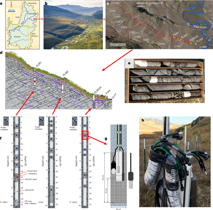
hydrosphere and atmosphere. The study was conducted in the Upper Colorado River Basin, East River watershed, along a lower montane hillslope underlain by Mancos Shale (Fig. 1a–e). On a

hillslope-to-floodplain flow transect (Fig. 1b–d), we drilled five boreholes 10 m deep into the bedrock, collecting rock cuttings and core samples (Fig. 1e). Three of the boreholes were

instrumented at different depths with sensors for measuring hydraulic potentials, moisture content and temperature (Fig. 1f,g) and samplers for collecting pore waters and pore gas (Fig. 1h)

over five years. Knowledge of weathering zone depths is crucial for quantifying weathering rates and C fluxes. In this Article we define the depth interval where weathering reactions are

most active22 as the ‘weathering zone’ (WZ), define its lower boundary where geochemical conditions support weathering as the ‘weathering front’ (WF) for specific rock components and the

zone below the WF as the ‘fractured bedrock’ (FBR). WATER TABLE DYNAMICS DRIVE SUBSURFACE FLOW The very high permeability of the hillslope soil accommodates infiltration from melting

snowpack, prevents overland flow and further supports the importance of subsurface flow on rock weathering22,33. Water mass balance was used to constrain recharge that drives groundwater

flow and reflects the competition between precipitation and evapotranspiration (ET) (Fig. 2a). Because ET from late spring through fall in this environment is high enough to prevent deep

infiltration from rainfall, recharge of groundwater only occurs during spring snowmelt and is incompletely drained from the WZ in high snowmelt years. Dissolved products of weathering are

removed in discharging waters, necessitating quantitative information on seasonal- and depth-dependent flow for calculating rates of bedrock weathering and solute transport. We calculated

water mass balances over five years with effective annual precipitation _P_e values (Methods) that optimize for interannual changes in subsurface water storage through carrying over

precipitation exceeding a threshold high snowpack water mass into the following year. Thus, on a water year (WY) basis, annual subsurface flow is equated with _P_e − ET (ref. 33). The water

table rises sharply during spring snowmelt, extending (in high snow years) into the soil, and declines to its lowest depths just before the following year’s snowmelt (Fig. 2b).

Gravity-driven subsurface flow within the hillslope depends on the elevation of the water table, hydraulic properties of each zone and the nearly constant water table slope, which remains

parallel to the soil surface. The transmissivity (_T_) within a given zone is its hydraulic conductivity (_K_) times its saturated thickness, and the transmissivity feedback model34 provides

a suitable representation for subsurface flow in many hillslopes such as ours where values of _K_ increase towards the soil surface. The values of _K_ for the soil and WZ and the value of

_T_ for the FBR were optimized so that calculated fluxes best matched _P_e _−_ ET over the course of five years (Methods). Daily groundwater flow rates through each zone (Fig. 2c) were

calculated based on the transmissivity feedback model and continuous water table elevation measurements (Fig. 2b). Flow through the FBR is relatively steady because it remains fully

saturated and the hydraulic gradient exhibits only minor fluctuations. Flow through the WZ oscillates annually in response to the continuously varying water table depth that drives

variations in its saturated thickness. The nonlinear dependence of flow on water table depth reflects the much higher _K_ values in the WZ and soil relative to the FBR. When snowmelt is

sufficient to raise the water table above the WZ, rapid downslope flow of shallow groundwater occurs along the soil. Although such periods with high water table are short (absent in low snow

years), they enable very high flow (up to 72% of the annual recharge) because of the high _K_soil. Annual partitioning of groundwater flow between the two months of maximum snowmelt and ten

‘baseflow’ months with lower discharge is shown in Supplementary Fig. 1a. These measurements of dynamic water table depths and stratified water fluxes make quantification of weathering

rates possible. QUANTIFYING CROCK WEATHERING RELEASE Three approaches were used to estimate rates of ICrock weathering: sulfate discharge, base cation discharge and eroded ICrock profile

reconstruction (Methods). The lowest estimate assumes that ICrock is only released in equimolar amounts with sulfate discharged upon pyrite oxidation. Time trends for sulfate concentrations

measured from pore-water samples were plotted for the three depth zones (Fig. 3a), which were then multiplied by their corresponding subsurface water fluxes (Fig. 2c) to obtain rates of

subsurface sulfate export within each zone and from the total subsurface (Fig. 3b). Export of sulfate and the other rock components in groundwater drives reactions (equations (1)–(4))

through removal of weathering products. Over the course of five years, sulfate was removed at a rate of 394 ± 267 kmol km−2 yr−1 with the ‘plus-minus’ values indicating standard deviations

among the five annual rates. The partitioning of exports for sulfate and other solutes between months of peak flow versus baseflow are shown in Supplementary Fig. 1, showing significant

dilution by snowmelt during high snowpack years and increased concentrations during baseflow. It should be noted that snowmelt includes solutes from the soil and WZ released above the water

table during the preceding baseflow interval. Whereas most of the acidity from pyrite dissolution drives ICrock dissolution, given that the ICrock:pyrite ratio of 4.26 mol mol−1 in the

unweathered bedrock (Extended Data Table 1) only slightly exceeds 4.027, a small fraction of acid from pyrite oxidation could contribute to silicate dissolution and C sequestration. The

second approach assumed that ICrock releases occur in proportion to its bedrock concentration relative to bedrock base cations (BC) concentration, given that BC export rates are often used

to quantify weathering rates35,36. Multiplying zone-specific pore water BC concentrations (Fig. 3c) by their corresponding subsurface water fluxes (Fig. 2c) yielded rates of BC exports

within each zone and for the total subsurface (Fig. 3d). Over the course of five years, a BC export of 1,420 ± 530 kmolc km−2 yr−1 was obtained, similar to rates reported for other

sedimentary watersheds36,37. On the basis of our measured ICrock:BCrock ratio of 0.32 mol molc−1, the BC-based estimate for ICrock release is 447 ± 170 kmol C km−2 yr−1. This estimate for

ICrock release is 13% greater than that obtained based on sulfate export, consistent with a small contribution from dissolution by carbonic acid. Reconstruction of the eroded ICrock depth

involved estimating the depleted sulfur solid phase inventory in the present profile (the yellow shaded area in Fig. 3e) and assuming the measured sulfate release rate of 394 kmol km−2 yr−1

(Fig. 3b) represents the average rate since recession of the Pinedale Glacier 16 thousand years ago (ka) (ref. 38). The total S removed over this time indicates that about 0.82 m of the

post-glacial regolith has eroded away. It is worth noting that the estimated 0.82 m of eroded regolith is equivalent to an erosion rate of 130 t km−2 yr−1, within the 42–420 t km−2 yr−1

range reported for slopes within the Rocky Mountains39,40. Adding the eroded thickness on the top of the current ICrock profiles (Fig. 3f) yields an ICrock release rate of 434 ± 41 kmol C 

km−2 yr−1 ( ± reflects uncertainty in timing of glacier retreat), remarkably similar to the rates obtained with the other two methods (Fig. 3, inserted table). It should be noted that the

depth for the ICrock WF is unclear in the solid phase profiles because of heterogeneous concentrations in unweathered rock and unknown contribution from precipitation of modern carbonates,

yet coincides with that of pyrite based on minima in pore water 14C profiles shown later. An OCrock release rate of 392 ± 37 kmol C km−2 yr−1 results from similarly adding the eroded

thickness on the top of the measured OCrock depletion profile (Fig. 3g). Because higher metamorphic grade or physical protection leaves a fraction of OCrock strongly resistant to

oxidation17,41,42, neither S nor BC exports were used to estimate OCrock oxidation. Whereas oxygen supply from water table lowering was the prerequisite for initiating weathering of pyrite,

ICrock and OCrock, differences in their initial concentrations and kinetics resulted in differences in their weathering profiles (Fig. 3e–g). Despite the overall slower oxidation rate of

OCrock relative to pyrite, pore-water depletion of 14C in dissolved organic carbon (DOC) profiles shown later support a WF depth for the more labile fraction of OCrock that coincides with

the WFs for pyrite and ICrock. Another metric for weathering at this East River hillslope was obtained from quantification of Si exports in pore waters, following the procedure described for

BC exports. The measured annual Si discharge rates of 16 to 69 kmol km−2 yr−1 (Supplementary Fig. 1h) are consistent with fluxes from other shale watersheds with similar precipitation and

run-off reported by Shaughnessy and Brantley43. QUANTIFYING EFFLUXES OF DIC, DOC AND CO2 Here exports of total C in porewaters and as CO2 are quantified, providing the context for Crock

releases into porewaters and gas presented in the next section. Time trends in pore-water dissolved inorganic carbon (DIC) concentrations within the three zones are shown in Fig. 4a. DIC

concentrations are highest in the WZ and FBR, reflecting weathering reactions and elevated partial pressure of CO2 (\(P_{{\rm{CO}}_2}\)) with depth and lowest in soil due to the depletion of

carbonate minerals and low \(P_{{\rm{CO}}_2}\). Multiplying the interpolated daily DIC concentrations within each zone by their respective Darcy fluxes (Fig. 2c) yields rates of DIC

discharge (Fig. 4b) and a total DIC export rate of 644 ± 307 kmol km−2 yr−1. Trends for DOC (Fig. 4c) show that the highest concentrations occur in soil, where modern organic carbon enters

the subsurface (next section). Export rates for DOC (Fig. 4d) were obtained by multiplying the interpolated daily concentrations within each zone by their corresponding flow rates (Fig. 2c),

resulting in a DOC export rate over five years of 98 ± 89 kmol km−2 yr−1. Diffusive losses of CO2 were calculated (Methods) based on seasonal changes in soil water content (Fig. 4e) and

temperature _T_ (Fig. 4f) that cause annual variations in the effective diffusion coefficient for CO2 at the soil surface (Fig. 4g). The time-dependent CO2 concentrations from the shallowest

soil gas samplers at the three locations (Fig. 4h) remain substantially elevated relative to the atmospheric CO2 concentration of about 420 ppm, especially under winter snowpack (yellow

background), which drives build-up of soil CO2. These CO2 concentrations together with other measured parameters (Fig. 4e–i) were used to calculate time-dependent diffusion rates (Fig. 4j).

Averaging the rates over the five years yielded a CO2 efflux of 4,000 ± 2,000 kmol C km−2 yr−1, within the range of soil respiration rates reported from similar environments44,45. As shown

next, this expected large CO2 efflux is predominantly Cmodern from soil respiration and is outside the scope of this study. RADIOCARBON DATA AND APPLICATIONS Radiocarbon (14C) relative

concentrations expressed as fraction modern (Fm) were determined in samples of solid OCbulk from soil to bedrock, DOC and DIC in depth-resolved pore waters and pore-gas CO2 (Methods). For

soil with shale as the parent material (shale fragments are abundant in soil), the OCbulk contains OCrock (Fm = 0) and biosphere OC (OCbio) (Fm ≤ 1). The measured Fmbulk from soil to bedrock

(Fig. 5a) indicate two end members and their depths: Fmbulk ≈ 1.0 at 0–0.05 m and Fmbulk = 0 at ≥2.0 m. Whereas ageing of OCbio occurs46,47, Fmbio values depend on the integrated rates of

OCbio formation and degradation. To estimate the Fmbio value above 2.0 m, we applied two approaches17,48 (Methods), and both support the approximation that Fm(OCbio) ≈ 1.0 in this system.

Fm(DOC) and Fm(DIC) values remain distinct in the three subsurface zones despite pore waters undergoing some mixing during flow (Fig. 5b,c). Fm(DOC) = 1.00 ( ± 0.03) in soil pore waters,

showing that the signature from OCrock weathering is overwhelmed by OCmodern release in the soil. The Fm(DIC and DOC) values decrease with depth to their minima at about 4 m (the WF),

showing Crock weathering occurs primarily in the WZ. Furthermore, these data provide the new insight that OCrock and ICrock share the same WF depth, despite having different weathering

rates. In pore-gas profiles (Fig. 5d), high rates of OCbio respiration keep Fm(CO2) ≈ 1.0 within soil, whereas Fm(CO2) values as low as 0.55 in the WZ demonstrate substantial transformation

of Crock to CO2. To calculate the Crock portion from the total C in groundwaters discharged from the hillslope, the average Fm(DOC) and Fm(DIC) in each depth zone (Fig. 5b,c inserted tables)

were weighted by their zone-specific flow rates (Fig. 2c) to obtain Fm discharge trends (Fig. 5e,f). The average Fm(DOC) = 0.81 ± 0.09 and Fm(DIC) = 0.79 ± 0.13 for waters discharged from

the hillslope ( ± indicate flow-weighted variation based on standard deviations of FM within each zone) and is consistent with hydrologic analyses showing that most of the snowmelt

discharges via shallow subsurface flow33,49. The broader watershed contains areas with and without shale bedrock49, resulting in higher Fm(DOC) = 0.94 ± 0.14 and Fm(DIC) = 0.86 ± 0.007 in

the river (Fig. 5b,c). The pore water Fm(DOC) and Fm(DIC) depth profiles (Fig. 5b,c) provide further support for the hypothesis that the lowest depth of annual oscillation water table

determines the depth of WF, previously based on shorter-term water table measurements and geochemical data22. As illustrated in Fig. 5g, the pyrite τ profiles (Methods) identified WF values

of 4.0, 4.2 and 3.3 for sites PLM 1, 2 and 3, respectively. These WF values are remarkably consistent with the water table depth minima at each of the locations (Fig. 5h). Through

integrating mineralogic, hydrologic and geochemical including radiocarbon analyses we revealed that weathering is most active in the subsurface zone exposed to the oscillating water table.

The water table minima can be used to predict the weathering front, shared by all the oxidation-dependent reactions (sulfide, ICrock and OCrock;Fig. 5b,c), with differences among reaction

rates reflected in depletion profiles (Fig. 3e–g). It is worth noting that kinetic limitations (including physical protection)6,50 and influx of oxygenated groundwaters27,51 contribute to

deviations from this pattern in other environments. Here reducing conditions observed below the water table22 indicate that microbial respiration depletes the diffusive supply of O2, thereby

preventing pyrite oxidation. DISCUSSION In this hillslope, Crock is released at the rate of 9.8 Mg km2 yr−1, with 82% emitted as CO2 (Fig. 6a). The remaining 18% is discharged through pore

waters, mostly as DICrock for later transformation to CO2 in oceans. All fluxes shown in this C balance diagram were calculated from measurements, except for the modern CO2 influx from

photosynthesis, which was assumed equal to the measured modern CO2 efflux from respiration. It should be noted that these two Cmodern rates are only included for completeness and do not

affect the absolute values of Crock flux calculations. It is also worth noting that release rates of rock CO2 are substantially lower in grey shales such as those of in the Shale Hills

catchment because of their low bedrock OCrock concentrations9. Given that the East River’s bedrock composition is typical of shales52, the representativeness of the hillslope’s Crock

releases can be evaluated through a comparison with estimates of global Crock weathering rates averaged per unit area. A comparison with global estimates of Crock fluxes from mountainous

areas is warranted given that these regions are considered primarily responsible for terrestrial Crock exports1,4,5,6,7,8,15. Estimates of global Crock releases range from 80 to 160 Mt yr−1

(refs. 1,6). Normalizing these estimates by the global terrestrial shale area5 of 3.42 × 107 km2, results in global average shale Crock release rates per unit area of 2.3 to 4.7 Mg km2 yr−1.

However, mountainous regions globally are the source for about 63% of discharge, while comprising only 32% of the terrestrial surface area53. Scaling the global average shale Crock release

rates by these factors leads to average shale Crock release rates from mountainous regions of 4.6 to 9.2 Mg km2 yr−1. These global and hillslope (9.8 Mg km2 yr−1) release rates are

remarkably consistent and support the broad importance of subsurface flow within oxidizing weathering zones for releasing Crock in mountainous regions. Whereas Ganges floodplain solute

release rates were found to be higher than those of their Himalayan source areas54, other studies have reported disproportionately greater weathering in mountainous watersheds1,4,5,6,7,8,15.

In such regions receiving higher precipitation, Crock releases may be more sensitive to climate change than the more areally extensive basin regions. Indeed, climate change is already

increasing the frequency of consecutive snow drought years55,56, a condition that will drive the water table deeper, into previously permanently saturated bedrock (Fig. 6b). Such water table

excursions deeper into the bedrock have been hypothesized to increase rates of oxidative weathering33,50. Whereas water table lowering will release more CO2(rock) to the atmosphere from

unsaturated bedrock, predicting its impacts on DICrock and DOCrock exports into rivers is challenging because these depend on recharge, which is projected to decrease under climate change57.

Nevertheless, Crock weathering and export are clearly controlled by climate via subsurface hydrologic regulation of oxygen availability and transport rates (Fig. 6b, Extended Data Fig. 1

and Extended Data Tables 2 and 3). The approaches used here can be applied in other environments, integrating chemical analyses of hillslope profiles with subsurface hydrological analyses to

further understand chemical weathering, weathering product exports into rivers and Crock contributions to the global C cycle. METHODS THE STUDY SITE The site is located 3.8 km

east–southeast of Snodgrass Mountain, Colorado, in the Rocky Mountains of the United States. The field study was conducted on a lower montane hillslope of the East River (ER) watershed

underlain by Mancos Shale, with intensive sampling and monitoring within the lower 140 m section of a transect that extends nearly 1 km to its peak (Fig. 1c). The hillslope drains into the

ER, which flows into the Gunnison River, a major tributary of the Colorado River. The ER contributes to 25% of the Gunnison River’s discharge, which in turn contributes to 40% of the

Colorado River’s discharge58,59. Cretaceous Mancos Shale is a dominant lithology in the region60, and solutes released by shale weathering strongly influence the chemistry of the ER Colorado

River waters60,61,62. The composition of the hillslope’s unweathered bedrock is typical of shales5,52,63, with 1.46 ± 0.40% ICrock and 1.53 ± 0.15% OCrock (including the kerogen hotspots),

4.1 ± 3.5% pyrite, 1.8 ± 2.2% calcite and 7.5 ± 1.6% dolomite22. The hillslope is vegetated with shallow rooted grasses and forbs, and its subsurface consists of 1.0 ± 0.3 m thick loam to

silt loam soil, underlain by weathered and fractured Mancos Shale bedrock. The area’s climate is continental subarctic, with a mean annual precipitation about 600 mm with about 70% as snow.

The ground is generally snow covered from November through early May, and monsoonal rains usually fall from mid‐July to September. BOREHOLE DRILLING AND INSTRUMENTATION Except for PLM6, all

the boreholes (0.254 m diameter) were drilled using waterless sonic drilling64, which allows drilling through the bedrock and recovery of depth-stratified samples of rock chips for

laboratory analyses. Soil samples were obtained within several metres of drilled boreholes, by coring (0.10 m diameter) to as deep as the hand-auger could be advanced, in 0.10 to 0.15 m

depth intervals. The average soil depth is 1.0 ± 0.3 m, based on 40 sampling holes along the hillslope. To track subsurface water flow and biogeochemical reactions, three of the five

boreholes (PLM 1, 2 and 3) were instrumented with sensors for measuring pressure, matric potential, moisture and temperature and samplers for collecting pore waters and pore gases65. The

outlets of the samplers are set about 1.5 m above the ground surface, designed for collecting pore-water and pore-gas samples even during the winter snow seasons. Through these instruments,

we obtained five years of time- and depth-dependent hydrologic and biogeochemical measurements of pore-water and pore-gas samples. It is worth noting that these pore-water, pore-gas and

solid samples retain highly localize chemistry, in contrast to samples from the river that integrate inputs from the whole watershed upstream of the collection point. The water table depths

were continuously recorded with pressure transducers (AquaTROLL 200) and also determined from equilibrium pressure measurements in pore-water samplers using the ‘tensisampler’ method66 and

from depth-distributed moisture sensors. SAMPLING OF DIFFERENT PHASES In the laboratory, a 4.75 mm sieve was used to remove roots and coarser gravel from soil samples. The rock samples were

collected at intervals of 50 cm and larger. All soil and the rock samples were oven dried at 105 °C for three days, then powdered to ≤50 µm for later analyses. Porewaters were collected with

depth-distributed suction/pressure samplers (Soilmoisture Equipment Corp., 1920F1L06-B02M2) biweekly in spring and monthly at other times except when the ground was frozen. The collected

water samples were filtered in the field through 0.45 µm polytetrafluoroethylene syringe filters (Pall, 0.45 µm). Each of the filtered water samples was divided into subsamples for different

types of analysis, including cation analysis (acidified immediately and stored in polyethylene vials), anion analysis, DOC and DIC analyses (collected in 40‐ml glass vials, filled to

eliminate headspace air). The water samples were kept in a cooler packed with coolant, shipped to the laboratory overnight and stored in a refrigerator for later analyses. Spatial

variability in solute concentrations within each zone reflects the fact that individual pore water sample volumes typically range from 100 to 200 ml, largely collected from regions extending

only several cm beyond the sampler’s intake surface67. Therefore, samplers embedded in locations undergoing more active weathering are generally expected to yield higher concentrations of

weathering products, whereas dilution from recharge waters (and from sulfate reduction) has the opposite effect68. Therefore, for each sampling time, solute concentrations obtained from

multiple samplers within a given zone were averaged to obtain representative values. The pore-gas samples were collected through custom-built pore-gas samplers65. At the field the extracted

gas from a specific depth was injected (slightly over-pressurized) through a 14 mm-thick chlorobutyl septa into a pre-evacuated 50 ml serum glass vial (Bellco Glass Inc.). SAMPLE ANALYSES

Soil and rock samples were analysed for elemental composition using X-ray fluorescence analyses by ALSGLOBAL-Geochemistry (http://www.alsglobal.com/geochemistry) in Reno, Nevada, United

States. The analyses were conducted under ALS (Australian Laboratory Systems) code numbers ME-XRF26 and ME-ICP61 for 33 elements using four acid digestions and inductively coupled plasma

atomic emission spectroscopy (ICP-AES), with uncertainty <0.1% based on three replicate measurements. Mineralogical compositions were determined by X-ray diffraction, by X-ray Mineral

Services (http://www.xrayminerals.co.uk) for both whole soil/rock samples and the clay fraction, with relative uncertainties <10%. Solid phase OC and IC were determined using a Shimadzu

TOC-VCSH total organic and inorganic carbon analyser in our LBNL/EESA Aqueous Geochemistry Laboratory, with relative uncertainty <1%. For pore-water samples, the major and trace element

cations were analysed using an inductively coupled plasma mass spectrometer (Thermo Fisher). The anions, Cl−, NO3−, NO2−, SO42−, PO43− were measured by ion chromatograph (Dionex, ICS‐2100,

Thermo Scientific USA) with precisions of ±5% of reported values. DOC and DIC were determined using a TOC-VCPH analyser (Shimadzu Corporation). DOC was analysed as non-purgeable organic

carbon by purging acidified samples with carbon-free air to remove DIC before measurement. For DOC and DIC measurements, relative standard deviation < 3% were estimated from 3–5

replicates. Pore-gas samples were analysed for CO2, N2O and CH4 concentrations using a Shimadzu Gas Chromatograph (GC-2014), with a precision of ±5% of the reported value. More details can

be found in our previous publications22,28,69. RADIOCARBON SAMPLING AND ANALYSES Subsamples from the same powdered soil and rock samples used for elemental and mineral composition analyses

were used for the analyses of 14C(OC) compositions in solid phase. For dissolved carbon, 14C(DOC) and 14C(DIC) in pore waters, large quantities of pore waters were required, relative to the

low volumetric yields of the pore-water samplers located above the water table. This is probably why data of this sort have not been previously available. Depending on carbon concentrations,

500 to 1,000 ml of pore water was needed for a sample. Below the water table, this quantity can be collected during a single sampling event. Above the water table, several successive

sampling events are required to collect sufficient volumes of pore waters for a single analysis. The 14C analyses in this paper are from several years of effort. 14C(DOC) water samples were

filtered and acidified in the field immediately after the collection with high purity hydrochloric acid to pH ~2.5 ± 0.3 and stored in glass bottles. 14C(DIC) samples were ‘poisoned’

immediately after sampling by adding saturated HgCl2 solution to kill the microorganisms and stored in glass bottles with no air space. Water samples were kept in a cooler with ice in the

field and stored in a refrigerator in the laboratory before analyses. River water samples were collected directly downslope of the flow transect, downstream of PLM4. The 14C(CO2) analyses in

gas phase requires 1 l of gas volume, collected in evacuated gastight 1,000-ml glass jars equipped with valves for connecting with the depth-distributed gas sampler outlets. Atmosphere air

samples were collected at the hillslope near PLM1. The solid phase 14C(OC) and gas phase 14C(CO2) were analysed by the W.M. Keck Carbon Cycle Accelerator Mass Spectrometer Facility at the

University of California, Irvine. Their protocols on sample preparation, analyses and reporting methods can be found at https://sites.uci.edu/keckams/protocols/. The compositions of

pore-water 14C(DOC) were analysed by the Woods Hole National Accelerator Mass Spectrometry Facility NOSAMS, following the protocols for sample preparation, analyses and data calculations at

https://www2.whoi.edu/site/nosams/radiocarbon-services/. The concentrations of pore-water 14C(DIC) were analysed by the Beta Analytics Radiocarbon Dating Service, and the method can be found

at https://www.betalabservices.com/biobased/carbon14-dating.html/. Solid, water and gas 14C results were corrected for isotopic fractionation according to the conventions of Stuiver and

Polach70, with δ13C values measured on prepared graphite using the accelerator mass spectrometer. Sample preparation backgrounds were subtracted based on measurements of 14C-free acid-washed

coal. The 14C concentrations are reported as fractions of the modern standard 14C (Fm), following the conventions of Stuiver and Polach70. WATER MASS BALANCE, SUBSURFACE FLOW AND SOLUTE

EXPORT To analyse water mass balance and determine subsurface water fluxes, we used daily precipitation (_P_) data from the Butte SNOTEL station71 located 3.1 km south of the site. Because

of interannual changes in subsurface water storage, annual subsurface flow is not simply equated with _P_ minute evapotranspiration (ET). Instead, subsurface flow on an annual basis was

equated with an effective annual precipitation (_P’_) minus ET. The influence of interannual subsurface water storage was approximated through allowing winter precipitation in excess of a

threshold level snowpack precipitation _P__tsp_ to contribute to effective precipitation in the following year. _P_tsp was set to 505 mm through optimizing the hillslope water mass balance

over five years with widely ranging annual _P_, resulting in 46 and 41 mm of _P_ from high snow water years 2017 and 2019 being carried over to water years 2018 and 2020, respectively33.

Correlations between air temperature data from the Butte SNOTEL station and ER-CSMWS were used to estimate the daily average, minimum and maximum air temperatures needed for calculating all

daily ET with the Community Land Model (CLM)72,73, except when snow cover was present. On days with snow covered ground, ET was assigned the average sublimation rate of 0.3 mm d−1 based on

eddy covariance measurements reported in a study conducted at a different mountainous location in Colorado74. The water table elevations continuously recorded by piezometers are shown in

Fig. 2b in the main text. Dividing the water table elevations between PLM1 and PLM3 locations by their horizontal separation distance of 137 m yields a continuous record of the hydraulic

gradient driving downslope flow. These measurements show that the flows are approximately parallel to the hillslope’s soil surface which has an average slope of 0.197 m m−1. Therefore, flow

within the saturated bedrock and variably saturated weathering zone and soil can be calculated using the Dupuit–Forchheimer approximation for flow along a sloping water table75 with the unit

normal area for groundwater flow being perpendicular to the slope. With this approximation, the cross-sectional area for flow is obtained through scaling down the saturated vertical

thickness by cos_θ_, where _θ_ is the slope between PLM1 and PLM3. With _θ_ = 11.2°, only a minor correction factor of cos_θ_ = 0.98 is needed because of the moderate slope. To calculate

downslope flow, the daily average water table elevations along the hillslope are used by determining the saturated thickness within the weathering zone (wz, 1.00–3.60 m average depth) _b_wz

and within the two soil regions (s1, 0–0.50 m depth and s2, 0.50–1.00 m depth) _b_s1 and _b_s2. Multiplying these cos_θ_-scaled thicknesses by the respective saturated _K_ assigned to each

layer, we obtained the respective transmissivities, _T_s1, _T_s2 and _T_wz. Note that the downslope flow along the soil is only effective when the water table resides within the soil such

that _b_si > 0, hence _T_s is usually zero. Very deep flow cannot be quantified because boreholes were only drilled to 10.0 m below ground surface. Therefore, the transmissivity of the

permanently saturated fractured bedrock _T_fbr was among the parameters adjusted to match the estimated annual subsurface flux. The daily subsurface flow equated to the sum of the four _T_

values times the hydraulic gradient (gradH), and these daily flows were summed to obtain yearly subsurface flow, _Q_a. $${Q}_\mathrm{a}=\mathop{\sum

}\limits_{\mathrm{day}\,1}^{\mathrm{day}\,365}\left({T}_\mathrm{s1}+{T}_\mathrm{s1}+{T}_{\mathrm{wz}}+{T}_{{\mathrm{f}}\;{\mathrm{br}}}\right)\mathrm{gradH}$$ (5) The subsurface water fluxes

were initially calculated with field-measured _K_s1, _K_s2, _K_wz and _K_fbr65. However, previous field studies showing that small-scale measurements substantially underestimate _K_ at the

hillslope scale76,77,78,79,80. On the basis of these considerations, all _K_ values were varied while keeping the depth _b_fbr at its original value to constraint the actual amounts of

flows. Additional constraints include that _K_s > _K_wz > _K_fbr, in keeping with original framework of the transmissivity feedback model. Daily water table-dependent

transmissivity-based fluxes for all layers were summed on a yearly basis for WY2017 through WY2021. Because the effective depth of the flow domain is unknown, _T_fbr rather than _K_fbr was

used for calculating flow through the bedrock. The variables _K_s1, _K_s2, _K_wz and _T_fbr were optimized using the Solver regression tool in Microsoft Excel. Adjusting these _K_, _T_ and

_P_tsp values to minimized deviations between annual calculated subsurface flow _Q_a and _P_e _−_ ET over the five years having widely varying _P_ yielded values of _K_s1, _K_s2 and _K_wz

equal to 1.4 \(\times\) 10−5, 2.7 \(\times\) 10−4 and 3.9 \(\times\) 10−6 m s−1, _T_fbr = 2.3 \(\times\) 10−6 m2 s−1 and _P_tsp = 508 mm, respectively. These optimized values resulted in a

small root mean-square deviation between _Q_a and _P_e _−_ ET of 43 mm (7% of the average annual _P_), despite encompassing years with near-record _P_ and drought years. Daily subsurface

discharges of solute species ‘_i_’ were calculated by weighting interpolated zone-specific concentrations by their corresponding daily flow rates

$${q}_{i}=\left({c}_{i,s1}{T}_{s1}+{c}_{i,s2}{T}_{s2}+{c}_{i,\mathrm{wz}}{T}_{\mathrm{wz}}+{c}_{i,\mathrm{fbr}}{T}_{\mathrm{fbr}}\right)\mathrm{gradH}$$ (6) Equation (6) shows how flow in

each active zone (when the water table height supports _b__i_ > 0, hence _T__i_ > 0) exerts a first-order impact on solute export. QUANTIFYING CROCK RELEASE RATES Three approaches were

used to estimate rates of ICrock weathering: sulfate discharge, base cation discharge and eroded ICrock profile reconstruction. Sulfate was not detectable in bedrock mineralogy nor in its

water extracts, and atmospheric deposition in the region contributes only about 0.4 kmol S km−2 yr−1 (ref. 81). Therefore, [SO42−] measured in pore waters is attributed to pyrite dissolution

in the weathering zone, and daily rates of [SO42−] discharge were calculated based on equation (6). Sulfate dissolution is assumed to release equivalent amounts of ICrock based on the much

higher dissolution rates of carbonate rocks relative to other minerals under acidic conditions7,8,35. Exports of base cations (BC = ∑(Na+, K+, Ca2+, Mg2+)) are often used to characterize

bedrock weathering, albeit indirectly from measurements in rivers35,36,37. We extended that method into the subsurface by tracking pore-water BC concentrations and flow within the soil, WZ

and FBR using equation (6). To estimate ICrock weathering based on BC export rates, we assumed that ICrock weathers in proportion to the measured ICrock:BCrock ratio of 0.32 mol molc−1. To

estimate the rate of ICrock release, the profiles of S (Fig. 3e) and ICrock (Fig. 3f) were assumed to reflect their weathering from Mancos Shale at constant rates, which for S is taken as

394 kmol km−2 yr−1 based on five years of sulfate discharge measurements. For reconstructing the pre-erosion regolith to determine past S and ICrock losses, time zero was assigned to the

retreat of the Pinedale Glacier from the hillslope, estimated at 16.0 ± 1.5 ka before present based on ages reported for neighbouring areas within the East River watershed38. Export of S

over 16.0 ± 1.5 ka at the average rate of 394 kmol km−2 yr−1 amounts to 6.30 ± 0.59 kmol m−2, equivalent to a bedrock weathering depth of 4.42 ± 0.41 m based on the unweathered shale S

concentration of 1.43 kmol m−3. Given the present-day S depletion depth of 3.60 m, about 0.82 ± 0.41 m of regolith has been eroded (Fig. 3e). The present-day weathering depleted ICrock

equivalent depth is then added to the 0.82 m of erosively removed regolith to estimated total ICrock released. Estimates of OCrock release were obtained with OCrock profiles, assuming OCrock

weathering release at constant rate over a period of 16.0 ± 1.5 ka. Combining the present-day OCrock depletion profile equivalent of 1.15 m unweathered shale with 0.82 m of erosively

removed regolith yields the estimated total OCrock released thickness of 1.97 m (Fig. 3g). The product of this total weathering thickness times the unweathered shale OCrock concentration of

3,180 mol m−3 was divided by 16,000 years to obtain the average OCrock release rate of 392 ± 37 kmol km−2 yr−1. QUANTIFYING CO2 DIFFUSION RATES Total porosities, matric potentials and

volumetric water contents (Fig. 4e) needed for calculating the effective diffusion coefficient were obtained from core sample measurements at adjacent locations and from sensors (Decagon 5TE

and MPS6), respectively82. Daily average soil temperature (Fig. 4f) measured by the shallowest matric potential sensor (Decagon MPS6) and an average local atmospheric pressure of 72 KPa

(estimated with the Boltzmann barometric equation for the average hillslope elevation of 2,776 m) were applied to Massman’s CO2 _D_o formula82,83. Specific values for _Φ_ for the midplane of

the shallowest interval at PLM1, PLM2 and PLM3 were assigned 0.58, 0.59 and 0.63, respectively, based on a polynomial fit of data on the depth dependence of shallow soil bulk densities and

an assumed solid density of 2.65 g cm−3. Values for the CO2 effective diffusion coefficient _D_e (Fig. 4g) were then calculated with the water-induced linear reduction model applied to

Marshall’s model84, $${D}_\mathrm{e}={D}_\mathrm{o}{\varepsilon }^{2.5}{\varPhi }^{{\rm{-}}1}$$ (7) where _Φ_ is the total porosity, _ε_ is the air-filled porosity (_Φ_ minus the volumetric

soil water content) and _D__o_ is the pressure- and temperature-dependent diffusion coefficient for CO2 in the bulk air phase. In the absence of snow cover, the CO2 concentrations measured

in the shallowest pore-gas samplers (Fig. 4h), and atmosphere samples were used to calculate the concentration gradient (Fig. 4i) for diffusion calculations based on Fick’s law82. During

winter time with snowpack, diffusive resistance within the snow cover causes CO2 concentrations to increase above 420 ppm at the soil–snow interface, and the interface CO2 concentration

requires estimation. For negligible storage within the snowpack, the diffusive fluxes of CO2 through the surface soil and snowpack are approximated as equal.

$${D}_\mathrm{e}\frac{\left({C}_{1}-{C}_\mathrm{b}\right)}{{z}_{1}}={D}_{\mathrm{snow}}\frac{\left({C}_\mathrm{b}-{C}_{0}\right)}{{z}_{2}}$$ (8) where _C_1, _C_b and _C_0 are the CO2

concentrations in the shallowest gas sampler (Fig. 4h), at the soil–snow boundary and in the atmosphere (420 ppm), respectively, _D_snow is the effective diffusion coefficient of CO2 through

snow, and _z__1_ and _z__2_ are the depth of the shallowest soil gas sampler and the thickness of the snowpack, respectively. Values of _D_snow were estimate based on the linear reduction

model (equation (7)), with _ε_ identical to _Φ_snow, using daily snow densities measured at the nearby snow telemetry station (Butte SNOTEL). The snowpack thicknesses _z__2_ were estimated

from a linear regression between measurements obtained along the hillslope transect during winters of 2017 and 2021, and thicknesses reported for the Butte SNOTEL. Values of _C_b were

calculated for steady-state diffusion in series through the surface soil and snowpack as

$${C}_\mathrm{b}=\left(\frac{{z}_{2}{D}_\mathrm{e}}{{z}_{1}{D}_{\mathrm{snow}}+{z}_{2}{D}_\mathrm{e}}\right){C}_{1}+\left(\frac{{z}_{1}{D}_{\mathrm{snow}}}{{z}_{1}{D}_{\mathrm{snow}}+{z}_{2}{D}_\mathrm{e}}\right){C}_{0}$$

(9) It should be noted that the calculated diffusive fluxes may be underestimates because wind can enhance gas fluxes through snow85. CO2 fluxes were calculated as the product of the _D_e

and the CO2 concentration gradient within the surface soil on a daily basis by applying Fick’s law. Daily diffusive fluxes based on a given gas sampling date were applied backwards and

forwards in time to midpoints between actual measurement days to interpolate between measured days. For the large data gap (September 2018 through May 2019) when samples were not available,

the average of all measured gradients was used for the location. Direct CO2 flux measurements were obtained during summer of 2018 with flux chambers (Li-Cor Biosciences LI-8100A) multiplexed

(LI-8150) to 0.203 m inner diameter collars embedded into the surface soils at three locations within each of the hillslope stations (PLM1, PLM2 and PLM3). The measurement system was

powered by a stationary set of batteries and solar panels, and flux chambers were moved sequentially to each of the PLM stations. At each of the stations, CO2 fluxes were cyclically measured

(measurement durations of 2 min, 20 min between measurements) on three collars over total run times of 3 to 5 days. It should be noted that recent studies indicates that flux chamber

measurements can yield overestimates of CO2 effluxes when steady-state conditions are not established86. QUANTIFYING CO2 LOSSES ORIGINATING FROM CROCK The total CO2 efflux originating from

Crock was obtained from the sum of ICrock and OCrock contributions. The rate of CO2 release originating from ICrock was calculated by subtracting the rate of DICrock export from the ICrock

weathering release rate. Likewise, the CO2 release originating from OCrock oxidation was calculated by subtracting the rate of DOCrock export from the OCrock weathering release rate.

CONTRIBUTION OF OCBIO AGEING At this site soil contains shallow roots and shale is the parent rock (Extended Data Fig. 1a shows unweathered shale fragments in soil). The soil contained OC is

a mixture of OCrock (Fmrock = 0) and biosphere OCbio (Fmbio ≤ 1.0, because OCbio starts ageing after its formation46,47). The very high OCbio% appear in the surface soil, where Fmbulk = 

1.0. The OCbio% together with Fmbulk rapidly decrease as the depth and reach to OCbio% = 0 and Fmbulk = 0 at depth about 2.0 m (Extended Data Fig. 1b,c). To estimate the Fmbio at the depth

above 2.0 m, we adapted two approaches by Galy et al.17 and Torres et al.48. They proposed that the particulates OC (POC) in riverine sediments are the mixture of ancient petrogenic OCrock

(Fmrock = 0.0) and OCbio (Fmbio values unknown) and derived models for estimating Fmbio values in riverine POC. Applying the approach of Galy et al.17

$${{\rm{Fm}}}_{{\rm{bulk}}}\times{{\rm{OC}}}_{{\rm{bulk}}} \% ={{\rm{Fm}}}_{{\rm{bio}}}\times{{\rm{OC}}}_{{\rm{bulk}}} \% -{{\rm{Fm}}}_{{\rm{bio}}}\times{{\rm{OC}}}_{{\rm{rock}}} \%$$ (10)

using measured Fmbulk and OCbulk%, we plotted the relations of Fmbulk × OCbulk% vs OCbulk% (Extended Data Fig. 1d). In this plot the data points from samples shallower than 2 m fall along a

single trendline (equation (11)) with _r_2 = 0.99, indicating mixing of two pure 14C end members. The data below about 2.0 m distribute along the _x_ axis, indicating 100% OCrock.

$${{Y}}=1.09{{X}}-1.05$$ (11) Comparing equations (10) and (11), we obtained Fmbio ≈ 1.09, showing that Fmbio is practically modern. The intercept value of −1.05 matches the OCrock% of the

bedrock at and below 2.0 m (Extended Data Fig. 1b). We also applied the approach from Torres et al.48 $${{\rm{Fm}}}_{{\rm{bulk}}}=[{{\rm{Fm}}}_{{\rm{b}}{\rm{io}}}{\times}({[{\rm{OC}} \%

]}_{{\rm{bulk}}}-{[{\rm{OC}} \% ]}_{{\rm{rock}}})]/{[{\rm{OC}} \% ]}_{{\rm{bulk}}}$$ (12) where Fmbulk, [OC%]bulk and [OC%]rock are measurements. Note that [OC]rock is represented by the

average in the bedrock (Extended Data Fig. 1b). The calculations resulted in Fmbio = 1.18 ± 0.10, again showed that Fmbio is practically modern. Whereas ageing of OCbio is certainly

occurring87, the integrated rates of its synthesis and degradation determines the overall age of accumulated OCbio. These analyses support the two end members mixing approach as a reasonable

approximation for this system. PYRITE RELATIVE CONCENTRATIONS The relative concentration τi,j2,88 defined by equation (13) for a given depth is used to evaluate loss of an element or

mineral relative to the unweathered parent rock caused by weathering $${\tau }_{i,\,j}=\frac{{{C}_{j,\mathrm{w}}C}_{i,\mathrm{p}}}{{{C}_{j,\mathrm{p}}C}_{i,\mathrm{w}}}-1$$ (13) where _c_

represents concentration, the subscript _j_ represents a mobile constituent (element or mineral of interest) and subscript _i_ represents the selected immobile reference element associated

with the parent rock. The subscripts w and p denote weathered and parent rock, respectively. In our calculations the pyrite concentrations in weathered and parent rock were measured depth

profiles from the three boreholes, PLM 1, 2 and 3. The value of parent rock pyrite concentration was determined by averaging the data at the depth below about 4.0 m from the three boreholes.

Titanium (Ti) was used as the immobile refs. 2,88. By following this approach, the weathering zone (WZ) can be defined as the depth region between −1 < τ < 0. The weathering front

(WF) is defined by the depth at which τ = 0. CALCULATING CROCK IN GROUNDWATER DISCHARGE Because large volumes of pore-water samples needed for 14C analyses could only be collected

infrequently, temporal trends of 14C Fm within the soil, weathering zone and bedrock pore waters were not obtained. Instead, average values of Fm(DOC) and Fm(DIC) within each of these zones

were used. Averages of Fm for DOC in soil, WZ and FBR are 0.95 ± 0.07, 0.51 ± 0.13 and 0.74 ± 0.11, respectively. Averages of 14C Fm for DIC measured in pore waters of soil, WZ and FBR are

0.97 ± 0.04, 0.77 ± 0.22 and 0.59 ± 0.08, respectively. These average FM were multiplied by daily flow rates within their corresponding zones to obtain flow-weighted overall 14C Fm of DOC

and DIC exported from the hillslope (Fig. 5e,f). Over the course of five years, the resulting average 14C Fm(DOC) and 14C Fm(DIC) are 0.81 ± 0.14 and 0.79 ± 0.08 respectively. HILLSLOPE

CARBON MASS BALANCE Essential background information used for determining fluxes of carbon in the hillslope and the component C influxes and effluxes and their measurement sources are

presented through three tables. Extended Data Table 1 summarizes average properties of the Mancos Shale bedrock, subsurface flow and weathering rates. Extended Data Tables 2 and 3 summarize

C influxes and effluxes, respectively. It should be noted that only the photosynthetic input of C included in Extended Data Table 2 is estimated (assuming balance with modern C effluxes),

and none of the other fluxes depend on that estimate. MAJOR SOURCES OF UNCERTAINTY Data needed for calculating weathering fluxes can be broadly categorized into chemical/mineralogical

analyses and hydrologic. Given that the chemical/mineralogical analyses involved in this study all follow standard procedures with quality control assuring small relative uncertainties

(generally much smaller than 5%), the greatest uncertainties in calculations are expected to be associated with hydrologic inputs. Given the central role of the hydrologic cycle in driving

weathering, the most basic uncertainties in modelling the processes presented here concern quantification of subsurface discharge, which in turn is determined from the differences between

precipitation and evapotranspiration. The details of that treatment were presented in Tokunaga et al.33 and the uncertainties are reviewed here. The Butte SNOTEL station, located 3 km away

from the hillslope site, was used for its continuous record of precipitation and other meteorological parameters needed for calculations of evapotranspiration. The next closest weather

station at Gothic, 5 km away in the opposite direction from the field site records precipitation amounts that are about 20% greater than those recorded at the Butte SNOTEL. Given that our

field site is approximately midway between the two weather stations and at an intermediate elevation, we expect that the uncertainty in daily precipitation for the site is about 10%. Unlike

measured precipitation, evapotranspiration (ET) rates were obtained from calculations based on the Community Land Model CLM73, with input parameters from the Butte SNOTEL and the hillslope

transect. Whereas the CLM has been widely used in a variety of environments, it is noteworthy that CLM-predicted ET agrees well with direct soil water mass balances measured at the East

River hillslope site33. Analyses of annual precipitation minus calculated annual ET showed that residual subsurface groundwater storage from high snowmelt years needs to be carried over to

the following water year to achieve consistent water mass balance. A carry-over of 46 mm (WY2017 into WY2018) and 41 mm (WY2019 into WY2020) combined with calibrating hydraulic conductivity

and transmissivity values optimized the total water mass balance, with a root mean-square deviation of 40 mm over the five water years. This deviation amounts to 24% of the average annual

discharge. Given the low porosity of snowpacks, the greatest uncertainties in diffusive CO2 fluxes are probably from possible wind-induced advection effects that could enhance releases

during periods with snow cover28. Given the greater diffusive resistance provided in the underlying soil zone, the wind-induced enhancement in CO2 efflux is not expected to exceed 10%. DATA

AVAILABILITY Data used in this paper have been placed in the US Department of Energy’s Environmental Systems Science Data Infrastructure for a Virtual Ecosystem (ESS-DIVE), accessible at

https://doi.org/10.15485/2322567. REFERENCES * Hilton, R. G. & West, A. J. Mountains, erosion and the carbon cycle. _Nat. Rev. Earth Env._ 1, 284–299 (2020). Article  CAS  Google Scholar

  * Anderson, S. P., Dietrich, W. E. & Brimhall, G. H. Weathering profiles, mass-balance analysis, and rates of solute loss: linkages between weathering and erosion in a small, steep

catchment. _Geol. Soc. Am. Bull._ 114, 1143–1158 (2002). Article  CAS  Google Scholar  * Wilson, M. J. Weathering of the primary rock-forming minerals: processes, products and rates. _Clay

Miner._ 39, 233–266 (2004). Article  CAS  Google Scholar  * Torres, M. A. et al. The acid and alkalinity budgets of weathering in the Andes-Amazon system: insights into the erosional control

of global biogeochemical cycles. _Earth Planet. Sci. Lett._ 450, 381–391 (2016). Article  CAS  Google Scholar  * Amiotte Suchet, P., Probst, J. L. & Ludwig, W. Worldwide distribution of

continental rock lithology: implications for the atmospheric/soil CO2 uptake by continental weathering and alkalinity river transport to the oceans. _Glob. Biogeochem. Cycles_ 17, 1038

(2003). Article  Google Scholar  * Petsch, S. T. in _Treatise on Geochemistry_ Vol. 12.8 (eds Turekian, K. & Holland, H.) 217–238 (Elsevier, 2014). * Torres, M. A., West, A. J. & Li,

G. J. Sulphide oxidation and carbonate dissolution as a source of CO2 over geological timescales. _Nature_ 507, 346 (2014). Article  CAS  PubMed  Google Scholar  * Calmels, D., Gaillardet,

J., Brenot, A. & France-Lanord, C. Sustained sulfide oxidation by physical erosion processes in the Mackenzie River basin: climatic perspectives. _Geology_ 35, 1003–1006 (2007). Article

  CAS  Google Scholar  * Jin, L. X. et al. The CO2 consumption potential during gray shale weathering: insights from the evolution of carbon isotopes in the Susquehanna Shale Hills critical

zone observatory. _Geochim. Cosmochim. Acta_ 142, 260–280 (2014). Article  CAS  Google Scholar  * Petsch, S. T., Edwards, K. J. & Eglinton, T. I. Microbial transformations of organic

matter in black shales and implications for global biogeochemical cycles. _Palaeogeogr. Palaeoclimatol. Palaeoecol._ 219, 157–170 (2005). Article  Google Scholar  * Hemingway, J. D. et al.

Microbial oxidation of lithospheric organic carbon in rapidly eroding tropical mountain soils. _Science_ 360, 209 (2018). Article  CAS  PubMed  Google Scholar  * Lerman, A., Wu, L. L. &

Mackenzie, F. T. CO2 and H2SO4 consumption in weathering and material transport to the ocean, and their role in the global carbon balance. _Mar. Chem._ 106, 326–350 (2007). Article  CAS 

Google Scholar  * Gabet, E. J. & Mudd, S. M. A theoretical model coupling chemical weathering rates with denudation rates. _Geology_ 37, 151–154 (2009). Article  CAS  Google Scholar  *

Hilton, R. G., Galy, A. & Hovius, N. Riverine particulate organic carbon from an active mountain belt: Importance of landslides. _Glob. Biogeochem. Cycles_

https://doi.org/10.1029/2006gb002905 (2008). * Das, A., Chung, C. H. & You, C. F. Disproportionately high rates of sulfide oxidation from mountainous river basins of Taiwan orogeny:

sulfur isotope evidence. _Geophys. Res. Lett._ https://doi.org/10.1029/2012gl051549 (2012). * Hilton, R. G. et al. Concentration-discharge relationships of dissolved rhenium in alpine

catchments reveal its use as a tracer of oxidative weathering. _Water Resour. Res_. https://doi.org/10.1029/2021WR029844 (2021). * Galy, V., Beyssac, O., France-Lanord, C. & Eglinton, T.

Recycling of graphite during himalayan erosion: a geological stabilization of carbon in the crust. _Science_ 322, 943–945 (2008). Article  CAS  PubMed  Google Scholar  * Tune, A. K.,

Druhan, J. L., Lawrence, C. R. & Rempea, D. M. Deep root activity overprints weathering of petrogenic organic carbon in shale. _Earth Planet. Sci. Lett._ 607, 118048 (2023). Article  CAS

  Google Scholar  * West, A. J. Thickness of the chemical weathering zone and implications for erosional and climatic drivers of weathering and for carbon-cycle feedbacks. _Geology_ 40,

811–814 (2012). Article  Google Scholar  * Brantley, S. L. et al. Toward a conceptual model relating chemical reaction fronts to water flow paths in hills. _Geomorphology_ 277, 100–117

(2017). Article  Google Scholar  * Lebedeva, M. I. & Brantley, S. L. Relating the depth of the water table to the depth of weathering. _Earth Surf. Processes Landforms_ 45, 2167–2178

(2020). Article  Google Scholar  * Wan, J. et al. Predicting sedimentary bedrock subsurface weathering fronts and weathering rates. _Sci. Rep._ https://doi.org/10.1038/s41598-019-53205-2

(2019). * Rempe, D. M. & Dietrich, W. E. Direct observations of rock moisture, a hidden component of the hydrologic cycle. _Proc. Natl Acad. Sci. USA_ 115, 2664–2669 (2018). Article  CAS

  PubMed  PubMed Central  Google Scholar  * Tune, A. K., Druhan, J. L., Wang, J., Bennett, P. C. & Rempe, D. M. Carbon dioxide production in bedrock beneath soils substantially

contributes to forest carbon cycling. _J. Geophys. Res. G: Biogeosci._ https://doi.org/10.1029/2020JG005795 (2020). * Salve, R., Rempe, D. M. & Dietrich, W. E. Rain, rock moisture

dynamics, and the rapid response of perched groundwater in weathered, fractured argillite underlying a steep hillslope. _Water Resour. Res._ 48, W11528 (2012). Article  Google Scholar  *

Anderson, S. P. & Dietrich, W. E. Chemical weathering and runoff chemistry in a steep headwater catchment. _Hydrol. Processes_ 15, 1791–1815 (2001). Article  Google Scholar  * Brantley,

S. L., Holleran, M. E., Jin, L. X. & Bazilevskaya, E. Probing deep weathering in the Shale Hills Critical Zone Observatory, Pennsylvania (USA): the hypothesis of nested chemical reaction

fronts in the subsurface. _Earth Surf. Processes Landforms_ 38, 1280–1298 (2013). Article  CAS  Google Scholar  * Wan, J. et al. Bedrock weathering contributes to subsurface reactive

nitrogen and nitrous oxide emissions. _Nat. Geosci._ 14, 217 (2021). Article  CAS  Google Scholar  * Soulet, G. et al. Temperature control on CO2 emissions from the weathering of sedimentary

rocks. _Nat. Geosci._ 14, 665–66 (2021). Article  CAS  Google Scholar  * Sullivan, P. L. et al. Oxidative dissolution under the channel leads geomorphological evolution at the Shale Hills

catchment. _Am. J. Sci._ 316, 981–1026 (2016). Article  CAS  Google Scholar  * Winnick, M. J. et al. Snowmelt controls on concentration-discharge relationships and the balance of oxidative

and acid-base weathering fluxes in an alpine catchment, East River, Colorado. _Water Resour. Res._ 53, 2507–2523 (2017). Article  CAS  Google Scholar  * Torres, M. A., West, A. J. &

Clark, K. E. Geomorphic regime modulates hydrologic control of chemical weathering in the Andes-Amazon. _Geochim. Cosmochim. Acta_ 166, 105–128 (2015). Article  CAS  Google Scholar  *

Tokunaga, T. K. et al. Quantifying subsurface flow and solute transport in a snowmelt-recharged hillslope with multiyear water balance. _Water Resour. Res._ 58, e2022WR032902 (2022). Article

  Google Scholar  * Bishop, K., Seibert, J., Nyberg, L. & Rodhe, A. Water storage in a till catchment. II: implications of transmissivity feedback for flow paths and turnover times.

_Hydrol. Processes_ 25, 3950–3959 (2011). Article  Google Scholar  * Langmuir, D. _Aqueous Environmental Geochemistry_ (Prentice-Hall, 1997). * Horton, T. W., Chamberlain, C. P., Fantle, M.

& Blum, J. D. Chemical weathering and lithologic controls of water chemistry in a high-elevation river system: Clark’s Fork of the Yellowstone River, Wyoming and Montana. _Water Resour.

Res._ 35, 1643–1655 (1999). Article  CAS  Google Scholar  * Anderson, S. P., Drever, J. I. & Humphrey, N. F. Chemical weathering in glacial environments. _Geology_ 25, 399–402 (1997).

Article  CAS  Google Scholar  * Quirk, B. J., Larsen, I. J. & Hidy, A. J. Latest Pleistocene glacial chronology and paleoclimate reconstruction for the East River watershed, Colorado,

USA. _Quat. Res._ 119, 86–98 (2024). Article  CAS  Google Scholar  * Smith, M. E., Carroll, A. R. & Mueller, E. R. Elevated weathering rates in the Rocky Mountains during the Early

Eocene Climatic Optimum. _Nat. Geosci._ 1, 370–374 (2008). Article  Google Scholar  * Foster, M. A., Anderson, R. S., Wyshnytzky, C. E., Ouimet, W. B. & Dethier, D. P. Hillslope lowering

rates and mobile-regolith residence times from in situ and meteoric Be-10 analysis, Boulder Creek Critical Zone Observatory, Colorado. _Geol. Soc. Am. Bull._ 127, 862–878 (2015). Article 

Google Scholar  * Wildman, R. A. et al. The weathering of sedimentary organic matter as a control on atmospheric O2: I. analysis of a black shale. _Am. J. Sci._ 304, 234–249 (2004). Article

  CAS  Google Scholar  * Gu, X. & Brantley, S. L. How particle size influences oxidation of ancient organic matter during weathering of black shale. _ACS Earth Space Chem._ 6, 1443–1459

(2022). Article  CAS  PubMed  PubMed Central  Google Scholar  * Shaughnessy, A. R. & Brantley, S. L. How do silicate weathering rates in shales respond to climate and erosion? _Chem.

Geol_. https://doi.org/10.1016/j.chemgeo.2023.121474 (2023). * Zhao, Z. Y. et al. Model prediction of biome-specific global soil respiration from 1960 to 2012. _Earth’s Future_ 5, 715–729

(2017). Google Scholar  * Raich, J. W. & Schlesinger, W. H. The global carbon-dioxide flux in soil respiration and Its relationship to vegetation and climate. _Tellus B_ 44, 81–99

(1992). Article  Google Scholar  * Lawrence, C. R., Harden, J. W., Xu, X. M., Schulz, M. S. & Trumbore, S. E. Long-term controls on soil organic carbon with depth and time: a case study

from the Cowlitz River Chronosequence, WA USA. _Geoderma_ 247, 73–87 (2015). Article  Google Scholar  * Torn, M. S., Trumbore, S. E., Chadwick, O. A., Vitousek, P. M. & Hendrick, D. M.

Mineral control of soil organic carbon storage and turnover. _Nature_ 389, 170–173 (1997). Article  CAS  Google Scholar  * Torres, M. A. et al. Model predictions of long-lived storage of

organic carbon in river deposits. _Earth Surf. Dyn._ 5, 711–730 (2017). Article  Google Scholar  * Carroll, R. W. H. et al. Factors controlling seasonal groundwater and solute flux from

snow-dominated basins. _Hydrol. Processes_ 32, 2187–2202 (2018). Article  Google Scholar  * Manning, A. H., Verplanck, P. L., Caine, J. S. & Todd, A. S. Links between climate change,

water-table depth, and water chemistry in a mineralized mountain watershed. _Appl. Geochem._ 37, 64–78 (2013). Article  CAS  Google Scholar  * Liao, R. X., Gu, X. & Brantley, S. L.

Weathering of chlorite from grain to watershed: the role and distribution of oxidation reactions in the subsurface. _Geochim. Cosmochim. Acta_ 333, 284–307 (2022). Article  CAS  Google

Scholar  * Copard, Y., Amiotte-Suchet, P. & Di-Giovanni, C. Storage and release of fossil organic carbon related to weathering of sedimentary rocks. _Earth Planet. Sci. Lett._ 258,

345–357 (2007). Article  CAS  Google Scholar  * Viviroli, D., Weingartner, R. & Messerli, B. Assessing the hydrological significance of the world’s mountains. _Mt. Res. Dev._ 23, 32–40

(2003). Article  Google Scholar  * Bickle, M. J. et al. Chemical weathering outputs from the flood plain of the Ganga. _Geochim. Cosmochim. Acta_ 225, 146–175 (2018). Article  CAS  Google

Scholar  * Marshall, A. M., Abatzoglou, J. T., Link, T. E. & Tennant, C. J. Projected changes in interannual variability of peak snowpack amount and timing in the western United States.

_Geophys. Res. Lett._ 46, 8882–8892 (2019). Article  Google Scholar  * Alvarez-Garreton, C., Boisier, J. P., Garreaud, R., Seibert, J. & Vis, M. Progressive water deficits during

multiyear droughts in basins with long hydrological memory in Chile. _Hydrol. Earth Syst. Sci._ 25, 429–446 (2021). Article  Google Scholar  * Miller, O. L. et al. How will baseflow respond

to climate change in the Upper Colorado River Basin? _Geophys. Res. Lett._ https://doi.org/10.1029/2021GL095085 (2021). * Ugland, R. C., Cochran, B. J., Kretschman, R. G., Wilson, E. A.

& Bennett, J. D. _Water Resources Data, Colorado, Water Year 1990, Vol. 2. Colorado River Basin_ Water Data Report CO-90-2 (US Geological Survey, 1991). * Spahr, N. E., Boulger, R. W.

& Szmajter, R. J. _Water Quality at Basic Fixed Sites in the Upper Colorado River Basin National Water-Quality Assessment Study Unit, October 1995–September 1998_ Water Resource

Investigations Report 99-4223 (US Geological Survey, 1999). * Morrison, S. J., Goodknight, C. S., Tigar, A. D., Bush, R. P. & Gil, A. Naturally occurring contamination in the Mancos

Shale. _Environ. Sci. Technol._ 46, 1379–1387 (2012). Article  CAS  PubMed  Google Scholar  * Winnick, M. et al. Snowmelt controls on concentration-discharge relationships and the balance of

oxidative and acid-base weathering fluxes in an alpine catchment, East River, Colorado. _Water Resour. Res._ 53, 2507–2523 (2017). Article  CAS  Google Scholar  * Carroll, R. W. H. et al.

Factors controlling seasonal groundwater and solute flux from snow‐dominated basins. _Hydrol. Processes_ 32, 2187–2202 (2017). Article  Google Scholar  * Shaw, D. B. & Weaver, C. E.

Mineralogical Composition of Shales. _J. Sediment. Petrol._ 35, 213–21 (1965). CAS  Google Scholar  * _Standard Practices for Sonic Drilling for Site Characterization and Installation of

Subsurface Monitoring Devices_ ASTM D 6914-04, 1-11 (ASTM, 2004). * Tokunaga, T. K. et al. Depth- and time-resolved distributions of snowmelt-driven hillslope subsurface flow and transport

and their contributions to surface waters. _Water Resour. Res._ 55, 9474–9499 (2019). Article  Google Scholar  * Tokunaga, T. The pressure response of the soil water sampler and

possibilities for simultaneous soil solution sampling and tensiometry. _Soil Sci._ 154, 171–183 (1992). Article  Google Scholar  * Wu, L., Baker, J. M. & Allmaras, R. R. Numerical and

field evaluation of soil water sampled by suction lysimeters. _J. Environ. Qual._ 24, 147–152 (1995). Article  CAS  Google Scholar  * Netto, A. M., Pieritz, R. A. & Gaudet, J. P. Field

study on the local variability of soil water content and solute concentration. _J. Hydrol._ 215, 23–37 (1999). Article  CAS  Google Scholar  * Wan, J. M. et al. Deep unsaturated zone

contributions to carbon cycling in semiarid environments. _J. Geophys. Res. Biogeosci._ 123, 3045–3054 (2018). Article  CAS  Google Scholar  * Stuiver, M. & Polach, H. A. Reporting of

C-14 data—discussion. _Radiocarbon_ 19, 355–363 (1977). Article  Google Scholar  * _Colorado SNOTEL Site Butte (380)_ (USDA, 2021); https://wcc.sc.egov.usda.gov/nwcc/site?sitenum=380 *

Oleson, K. W. et al. _Technical Description of Version 4.5 of the Community Land Model (CLM)_ 434 (National Center for Atmospheric Research, 2013). * Tran, A. P., Rungee, J., Faybishenko,

B., Dafflon, B. & Hubbard, S. S. Assessment of spatiotemporal variability of evapotranspiration and its governing factors in a mountainous watershed. _Water_ 11, 243 (2019). Article 

Google Scholar  * Sexstone, G. A., Clow, D. W., Stannard, D. I. & Fassnacht, S. R. Comparison of methods for quantifying surface sublimation over seasonally snow-covered terrain.

_Hydrol. Processes_ 30, 3373–3389 (2016). Article  Google Scholar  * Childs, E. C. Drainage of groundwater resting on a sloping bed. _Water Resour. Res._ 7, 1256–1263 (1971). Article  Google

Scholar  * Brooks, E. S., Boll, J. & McDaniel, P. A. A hillslope-scale experiment to measure lateral saturated hydraulic conductivity. _Water Resour. Res._ 40, W04208 (2004). Article 

Google Scholar  * Di Prima, S., Marrosu, R., Lassabatere, L., Angulo-Jaramillo, R. & Pirastru, M. In situ characterization of preferential flow by combining plot- and point-scale

infiltration experiments on a hillslope. _J. Hydrol._ 563, 633–642 (2018). Article  Google Scholar  * Glaser, B., Jackisch, C., Hopp, L. & Klaus, J. How meaningful are plot-scale

observations and simulations of preferential flow for catchment models? _Vadose Zone J._ 18, 180146 (2019). Article  Google Scholar  * Uchida, T., Kosugi, K. & Mizuyama, T. Effects of

pipeflow on hydrological process and its relation to landslide: a review of pipeflow studies in forested headwater catchments. _Hydrol. Processes_ 15, 2151–2174 (2001). Article  Google

Scholar  * Wilson, G. V., Rigby, J. R., Ursic, M. & Dabney, S. M. Soil pipe flow tracer experiments: 1. connectivity and transport characteristics. _Hydrol. Processes_ 30, 1265–1279

(2016). Article  Google Scholar  * _CASTNET_ (US EPA, 2019). * Tokunaga, T. K. et al. Deep vadose zone respiration contributions to carbon dioxide fluxes from a semiarid floodplain. _Vadose

Zone J._ https://doi.org/10.2136/vzj2016.02.0014 (2016). * Massman, W. J. A review of the molecular diffusivities of H2O, CO2, CH4, CO, O-3, SO2, NH3, N2O, NO, and NO2 in air, O2 and N2 near

STP. _Atmos. Environ._ 32, 1111–1127 (1998). * Moldrup, P. et al. Predicting the gas diffusion coefficient in repacked soil: water-induced linear reduction model. _Soil Sci. Soc. Am. J._

64, 1588–1594 (2000). Article  CAS  Google Scholar  * Bowling, D. R. & Massman, W. J. Persistent wind-induced enhancement of diffusive CO2 transport in a mountain forest snowpack. _J.

Geophys. Res. Biogeosci._ https://doi.org/10.1029/2011jg001722 (2011). * Braendholt, A., Larsen, K. S., Ibrom, A. & Pilegaard, K. Overestimation of closed-chamber soil CO2 effluxes at

low atmospheric turbulence. _Biogeosciences_ 14, 1603–1616 (2017). Article  CAS  Google Scholar  * Shi, Z. et al. The age distribution of global soil carbon inferred from radiocarbon

measurements. _Nat. Geosci._ 13, 555–55 (2020). Article  CAS  Google Scholar  * Brimhall, G. H. & Dietrich, W. E. Constitutive mass balance relations between chemical-composition,

volume, density, porosity, and strain in metasomatic hydrochemical systems—results on weathering and pedogenesis. _Geochim. Cosmochim. Acta_ 51, 567–587 (1987). Article  CAS  Google Scholar

  Download references ACKNOWLEDGEMENTS We thank Rocky Mountain Biological Laboratory (RMBL) for helping with field research, J. L. Druhan for an internal review of the manuscript and S.

Brantley for reviews and constructive comments. This work was conducted as part of the Watershed Function Scientific Focus Area at Lawrence Berkeley National Laboratory and was supported by

the US Department of Energy (DOE) Environmental System Science Research Program, DOE Office of Science, Office of Biological and Environmental Research, under contract number DE-AC02 − 

05CH11231. Mention of trade names and commercial analytical services does not imply endorsement. AUTHOR INFORMATION AUTHORS AND AFFILIATIONS * Earth and Environment Sciences Area, Lawrence

Berkeley National Laboratory, Berkeley, CA, USA Jiamin Wan, Tetsu K. Tokunaga, Wenming Dong, Markus Bill & Kenneth H. Williams * Rocky Mountain Biological Laboratory, Crested Butte, CO,

USA Curtis A. Beutler, Alexander W. Newman, Wendy S. Brown, Amanda N. Henderson & Kenneth H. Williams * Water Resources Institute, Hanoi, Vietnam Anh Phuong Tran Authors * Jiamin Wan

View author publications You can also search for this author inPubMed Google Scholar * Tetsu K. Tokunaga View author publications You can also search for this author inPubMed Google Scholar

* Curtis A. Beutler View author publications You can also search for this author inPubMed Google Scholar * Alexander W. Newman View author publications You can also search for this author

inPubMed Google Scholar * Wenming Dong View author publications You can also search for this author inPubMed Google Scholar * Markus Bill View author publications You can also search for

this author inPubMed Google Scholar * Wendy S. Brown View author publications You can also search for this author inPubMed Google Scholar * Amanda N. Henderson View author publications You

can also search for this author inPubMed Google Scholar * Anh Phuong Tran View author publications You can also search for this author inPubMed Google Scholar * Kenneth H. Williams View

author publications You can also search for this author inPubMed Google Scholar CONTRIBUTIONS J.W. and T.K.T. designed and conducted part of the field and laboratory work and wrote the

manuscript. C.A.B., A.W.N., W.S.B. and A.N.H. conducted the field work. W.D. and M.B. conducted part of the laboratory chemical analyses. A.P.T. modelled ET. K.H.W. conducted and supervised

the field work. CORRESPONDING AUTHORS Correspondence to Jiamin Wan or Tetsu K. Tokunaga. ETHICS DECLARATIONS COMPETING INTERESTS The authors declare no competing interests. PEER REVIEW PEER

REVIEW INFORMATION _Nature Water_ thanks the anonymous reviewers for their contribution to the peer review of this work. ADDITIONAL INFORMATION PUBLISHER’S NOTE Springer Nature remains

neutral with regard to jurisdictional claims in published maps and institutional affiliations. EXTENDED DATA EXTENDED DATA FIG. 1 CONTRIBUTION OF OCBIO AGING. (A) Photograph of a soil core

cross section at about 1.0 m, showing rock fragments at the Soil-WZ interface. (B) Depth profiles of solid phase OCbulk%. (C) Depth profiles of Fmbulk. (D) Plots of Fmbulk * OCbulk% vs.

OCbulk%. SUPPLEMENTARY INFORMATION SUPPLEMENTARY INFORMATION Supplementary text and Fig. 1. RIGHTS AND PERMISSIONS OPEN ACCESS This article is licensed under a Creative Commons

Attribution-NonCommercial-NoDerivatives 4.0 International License, which permits any non-commercial use, sharing, distribution and reproduction in any medium or format, as long as you give

appropriate credit to the original author(s) and the source, provide a link to the Creative Commons licence, and indicate if you modified the licensed material. You do not have permission

under this licence to share adapted material derived from this article or parts of it. The images or other third party material in this article are included in the article’s Creative Commons

licence, unless indicated otherwise in a credit line to the material. If material is not included in the article’s Creative Commons licence and your intended use is not permitted by

statutory regulation or exceeds the permitted use, you will need to obtain permission directly from the copyright holder. To view a copy of this licence, visit

http://creativecommons.org/licenses/by-nc-nd/4.0/. Reprints and permissions ABOUT THIS ARTICLE CITE THIS ARTICLE Wan, J., Tokunaga, T.K., Beutler, C.A. _et al._ Hydrological control of rock

carbon fluxes from shale weathering. _Nat Water_ 2, 848–862 (2024). https://doi.org/10.1038/s44221-024-00293-8 Download citation * Received: 16 January 2024 * Accepted: 18 July 2024 *

Published: 26 August 2024 * Issue Date: September 2024 * DOI: https://doi.org/10.1038/s44221-024-00293-8 SHARE THIS ARTICLE Anyone you share the following link with will be able to read this

content: Get shareable link Sorry, a shareable link is not currently available for this article. Copy to clipboard Provided by the Springer Nature SharedIt content-sharing initiative